Shape Up Your Maps with Shapefiles

Add custom features using polygons, points, and lines

Familiarity with shapefiles is essential for working with geospatial data. These specialized datasets enable the placement of custom shapes on maps and are surprisingly easy to use.

While Python’s third-party geospatial libraries contain useful built-in datasets, such as country outlines, their utility is limited. If you need to plot and emphasize other features, such as city boundaries or the extent of English dialects in the UK, you’ll need a custom shapefile. In this Quick Success Data Science project, we’ll use a shapefile and the GeoPandas library to highlight and explore some of the world’s largest lakes.

The GeoPandas Library

GeoPandas is an open-source, third-party library designed to support geospatial mapping in Python. It extends the datatypes used by the pandas library and makes working with geospatial vector data similar to working with tabular data. It also enables operations in Python that would otherwise require a dedicated geospatial database, such as Post GIS.

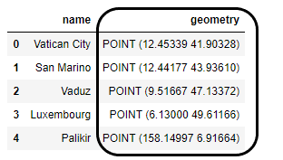
A GeoDataFrame is a pandas DataFrame with a special “geometry” column for location data. This column bundles together the type of geometric object (such as a point, line string, polygon, etc.) and the coordinates (longitude and latitude) needed to draw it.

GeoPandas relies on several other libraries such as Shapely for planar geometric shapes (like street centerlines); Fiona for reading and writing geographical data file formats; pyproj for handling projections; matplotlib for plotting; and descartes for integrating Shapely geometry objects with matplotlib. Shapely is also used to perform geometric operations. Given all this support, it’s no wonder that GeoPandas is Python’s most popular library for parsing geospatial data.

To install GeoPandas, just run the following:

conda install geopandas

or

pip install geopandas

Shapefiles

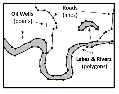
A shapefile is a geospatial vector data format for geographic information system (GIS) software. This format can spatially describe vector features such as points, lines, and polygons. Each item in the file usually includes descriptive attributes, such as a name.

Despite its name, a “shapefile” isn’t a single file but a collection of files in a single folder. The figure below shows the shapefile we’ll use for this project. Note how all of the filenames use the folder name as a prefix.

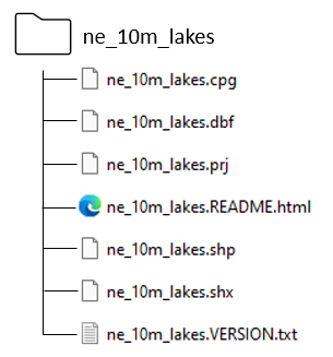
Three files are mandatory and have filename extensions of .shp, .shx, and .dbf. While the actual shapefile relates specifically to the .shp file, the other supporting files are required for capturing the shape geometry. For more detail on these files, check out the Wikipedia page on shapefiles.

Here’s the fun part. To use this collection of files, all we need to do is provide the directory path to the shapefiles folder (zipped or unzipped). GeoPandas knows how to work with the files in this folder to automatically produce the geometry column in the GeoDataFrame.

The Lakes Shapefile

There are multiple ways to make a shapefile from scratch, but the most common method is to use GIS software like ArcGIS or QGIS. Before trying to create your own shapefile, however, it’s wise to see if one already exists. After all, the sum of humankind’s knowledge resides on the internet, so it’s always worth a try. We should be able to find many sources for something as common as the outline of lakes.

For this project, we’ll use a shapefile from naturalearthdata.com. This file contains a crazy number of lakes, but we only want the most important ones, which can be identified using the shapefile’s scalerank parameter, which will become a column in our GeoDataFrame.

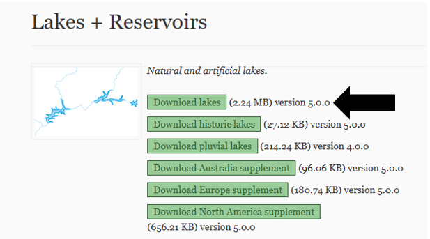
To download the shapefile, go to the Natural Earth website and click on the green “Download lakes” button shown below. This will download a zipped folder, which you can use directly, without the need for extraction. This is a nice feature as zipped folders are memory efficient.

Importing Libraries and Loading the Data

The only library we need to import for this project is GeoPandas.

To load the shapefile as a GeoDataFrame, we’ll use the GeoPandas read_file() method and pass the directory path to the ne_10m_lakes.zip folder. Of course, you’ll need to replace my path with your own.

import geopandas as gpd

# Load a shape file of world lakes as a GeoDataFrame:
path = r'C:\Users\hanna\quick_success\lakes\data\ne_10m_lakes.zip'
world_lakes = gpd.read_file(path)
world_lakes.head(3)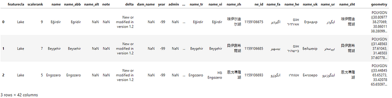

The resulting GeoDataFrame has many columns of data, but the only ones we need are the scalerank, name, and geometry columns.

Copying Out the Important Lakes

According to Natural Earth website, the scalerank column is the rank of each lake by relative importance, coordinating with river ranking. The most important lakes have a rank of 0. To choose these lakes, we'll make a new GeoDataFrame, named large_lakes, that includes rows from the previous GeoDataFrame that meet this criterion. While we're at it, we'll drop the columns that we don't need.

# Make new GeoDataFrame of important lakes using the "scalerank" column:
large_lakes = (world_lakes[world_lakes['scalerank'] == 0]
               [['scalerank', 'name', 'geometry']].reset_index(drop=True))
display(large_lakes)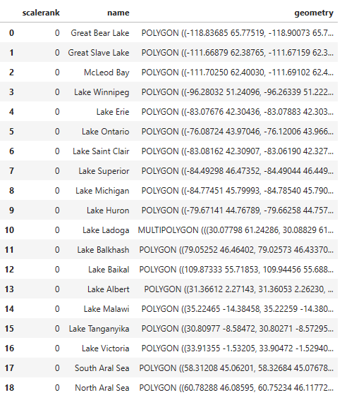

Note: For you geographers and lake fans, several large lakes, like Lake Turkana (formerly Lake Rudolf) and the Caspian Sea, are missing from this list. This is most likely due to the ranking system used by Natural Earth, which is based on the vague concept of “importance”. Since this article focuses on shapefiles rather than limnology, we’re going to ignore these issues moving forward.

Plotting the Lakes

GeoPandas ships with the naturalearth_lowres dataset, which produces a map of the world complete with country outlines. In order to overlay our lake data on this world map, we'll need to use the same matplotlib axes object (ax) for both datasets. We’ll pass this object in the last line when we call the GeoPandas plot() method on the large_lakes dataset.

# Plot the lakes on GeoPandas' built-in world map:
world = gpd.read_file(gpd.datasets.get_path('naturalearth_lowres'))
world = world[(world.name != 'Antarctica')]  # Leave off Antarctica
ax = world.plot(color='lightgray', figsize=(10, 10))
ax.set_title("Important Lakes of the World", fontsize=14)
large_lakes.plot(ax=ax, color='darkblue');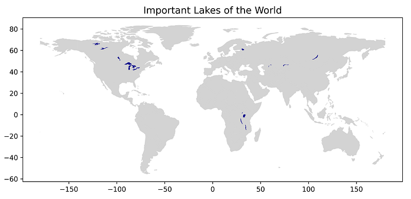

You’ve got to admit, that was quick and easy. Go, shapefiles!

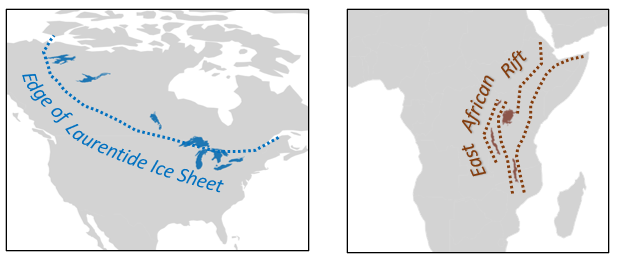
If you look closely at the map, you’ll notice that the large lakes in North America and Africa conform to linear patterns. This is not a chance occurrence, but a byproduct of their origin.

Color-coding Lakes by Their Mode of Origin

Let’s investigate the mode of origin for the world’s important lakes. As you can imagine, it takes a big event to make a big lake.

The majority of the world’s large lakes are the result of glaciation during the ice ages. Ice sheets gouged out valleys and pressed the crust down with their enormous weight. The Great Lakes owe their origin to heavy ice sheets and are currently growing shallower as the crust recovers from the load, a process called “isostatic rebound.”

Other lakes formed through the process of rifting, which occurs when continental plates pull apart. The relatively young East African Rift System, for example, is a nascent ocean currently occupied by huge freshwater lakes such as Lake Victoria.

A few of the Asian lakes represent tectonic “troughs” that form during the process of mountain-building. The true shape of these lakes has been significantly altered by human activity (see Aral Sea).

To transfer this information to our map, we’ll start by making a Python dictionary. The lake names will serve as the dictionary’s keys. These names should exactly conform to those used in the name column in the GeoDataFrame, as we’ll use them to match and merge the two datasets.

origin_type = {'Lake Superior': 'glacial', 
               'Lake Michigan': 'glacial', 
               'Lake Huron': 'glacial',
               'Lake Erie': 'glacial', 
               'Lake Ontario': 'glacial', 
               'Great Bear Lake': 'glacial',
               'Great Slave Lake': 'glacial', 
               'McLeod Bay': 'glacial', 
               'Lake Winnipeg': 'glacial',
               'Lake Saint Clair': 'glacial', 
               'Lake Ladoga': 'glacial', 
               'Lake Baikal': 'rift valley', 
               'Lake Albert': 'rift valley', 
               'Lake Malawi': 'rift valley',
               'Lake Tanganyika': 'rift valley', 
               'Lake Victoria': 'rift valley', 
               'Lake Balkhash': 'tectonic depression',
               'South Aral Sea': 'tectonic depression',
               'North Aral Sea': 'tectonic depression'}

Merging the Data

Before adding the dictionary to the GeoDataFrame, we’ll make a copy of the GeoDataFrame named large_lakes_2. In this new GeoDataFrame, we'll make a column for the origin type and use the map() method to merge it with the dictionary. This method will match the values in the name column to the keys in the dictionary.

# Make a new GeoDataFrame with a column for the type of origin:
large_lakes_2 = large_lakes.copy()
large_lakes_2['origin type'] = large_lakes_2['name'].map(origin_type)
large_lakes_2.tail(3)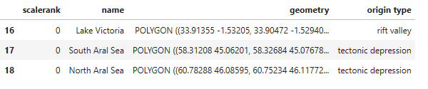

Plotting the Mode of Origin

Now we’ll run our plotting code again and pass origin type as the column argument.

# Plot the largest lakes color-coded for origin type:
ax = world.plot(color='lightgray', figsize=(10, 10))
ax.set_title("Mode of Origin of Important Lakes", fontsize=14)
large_lakes_2.plot(ax=ax, 
                   column=large_lakes_2['origin type'], 
                   legend=True);

# # Add names:
# large_lakes_2.apply(lambda x: ax.annotate(text=x['name'], 
#                                           xy=x.geometry.centroid.coords[0], 
#                                           ha='center', 
#                                           fontsize=6), axis=1);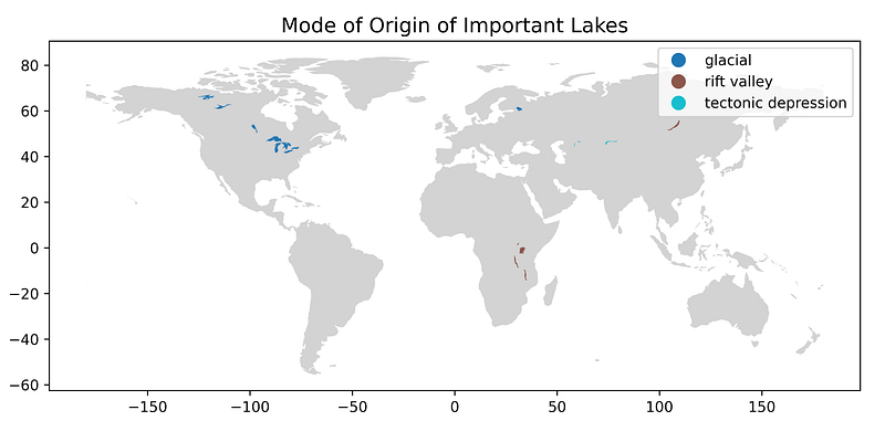

As you might expect, the glacial lakes are found in the north and the ones in North America “line up” with the extent of major ice sheets, such as the Laurentide Ice Sheet. Similar linearity occurs in Africa, where lakes formed in parallel grabens (downfaulted crustal blocks) within the East African Rift System.

Summary

Shapefiles are used to add vector data, such as polygons, lines, and points, to maps. These shapes can represent mappable features like bodies of water, roads, water sample locations, school district boundaries, the extent of ash falls from the Yellowstone supervolcano, and so on.

Shapefiles represent a collection of files, rather than a single file, and Python’s GeoPandas library is designed to work with them easily. All you need to do is point GeoPandas to the shapefile folder and it will automatically build a plottable GeoDataFrame of the data. Within the GeoDataFrame, the geometry column facilitates plotting the shapes on a map.

Most shapefiles are created using GIS software like ArcGIS and QGIS, but as you saw, you can edit them in GeoDataFrames. In this project, we added a column for the mode of origin of each large lake and then plotted the result.

Thanks!

Thanks for reading! If you found this article useful, then follow me for more Quick Success Data Science projects in the future.