avataragus abdul rahman

Free AI web copilot to create summaries, insights and extended knowledge, download it at here

4547

Abstract

t, which you can download from Kaggle</a>. The dataset looks clean, and the target column is <code>machine failure.</code> Before training a model, it’s essential to explore the data, handle any missing values, and perform feature engineering to improve predictive performance.</p><div id="51c1"><pre><span class="hljs-keyword">import</span> shap <span class="hljs-keyword">import</span> numpy <span class="hljs-keyword">as</span> np <span class="hljs-keyword">import</span> pandas <span class="hljs-keyword">as</span> pd

df = pd.read_csv(<span class="hljs-string">"./dataset/machine failure.csv"</span>) column_selected = [<span class="hljs-string">'Air temperature [K]'</span>, <span class="hljs-string">'Process temperature [K]'</span>, <span class="hljs-string">'Rotational speed [rpm]'</span>, <span class="hljs-string">'Torque [Nm]'</span>, <span class="hljs-string">'Tool wear [min]'</span>, <span class="hljs-string">'TWF'</span>, <span class="hljs-string">'HDF'</span>, <span class="hljs-string">'PWF'</span>, <span class="hljs-string">'OSF'</span>, <span class="hljs-string">'RNF'</span>, <span class="hljs-string">'Machine failure'</span>]

df = df[column_selected] df.head()

<span class="hljs-comment"># Convert data types to float</span> df = df.astype(<span class="hljs-built_in">float</span>)</pre></div><figure id="9782"><img src="https://cdn-images-1.readmedium.com/v2/resize:fit:800/1*PulTh0K5vsDJ1IoD-LSrPA.png"><figcaption>Image by Author</figcaption></figure><p id="9552"><b>Plot Correlation Matrix</b></p><div id="798e"><pre><span class="hljs-keyword">import</span> matplotlib.pyplot <span class="hljs-keyword">as</span> plt <span class="hljs-keyword">import</span> seaborn <span class="hljs-keyword">as</span> sns

corr_matrix = df.corr()

plt.figure(figsize=(<span class="hljs-number">10</span>, <span class="hljs-number">8</span>)) sns.heatmap(corr_matrix, annot=<span class="hljs-literal">True</span>, cmap=<span class="hljs-string">'coolwarm'</span>, linewidths=<span class="hljs-number">0.5</span>)

plt.title(<span class="hljs-string">"Corelation Matrix"</span>)</pre></div><figure id="1874"><img src="https://cdn-images-1.readmedium.com/v2/resize:fit:800/1*tb_8eTJ7P3Lioa99-txT3Q.png"><figcaption>Image by Author</figcaption></figure><h1 id="09bb">Model Training and Evaluation</h1><ol><li>Create X and y using a target column and split the dataset into train and test.</li><li>Train Random XGBClassifier on the training set.</li><li>Make predictions using a testing set.</li></ol><div id="9f9a"><pre><span class="hljs-keyword">from</span> xgboost <span class="hljs-keyword">import</span> XGBClassifier <span class="hljs-keyword">from</span> sklearn.metrics <span class="hljs-keyword">import</span> classification_report <span class="hljs-keyword">from</span> sklearn.metrics <span class="hljs-keyword">import</span> accuracy_score, f1_score <span class="hljs-keyword">from</span> sklearn.model_selection <span class="hljs-keyword">import</span> train_test_split

X = df[[<span class="hljs-string">'air_temperature__k_'</span>, <span class="hljs-string">'process_temperature__k_'</span>, <span class="hljs-string">'rotational_speed__rpm_'</span>, <span class="hljs-string">'torque__nm_'</span>, <span class="hljs-string">'tool_wear__min_'</span>, <span class="hljs-string">'twf'</span>, <span class="hljs-string">'hdf'</span>, <span class="hljs-string">'pwf'</span>, <span class="hljs-string">'osf'</span>]]

y = df[<span class="hljs-string">'machine_failure'</span>] <span class="hljs-comment"># Dependent variable</span>

<span class="hljs-comment"># Split into train and test </span> X_train, X_test, y_train, y_test = train_test_split(X, y, test_size=<span class="hljs-number">0.3</span>, random_state=<span class="hljs-number">1</span>)

<span class="hljs-comment"># Train an XGBoost model</span> model = XGBClassifier(n_estimators=<span class="hljs-number">100</span>, random_state=<span class="hljs-number">42</span>, use_label_encoder=<span class="hljs-literal">False</span>, eval_metric=<span class="hljs-string">'logloss'</span>) model.fit(X_train, y_train)

<span class="hljs-comment"># Predictions</span> y_pred = model.predict(X_test)

<span class="hljs-comment"># Evaluate model</span> accuracy = accuracy_score(y_test, y_pred) f1 = f1_score(y_test, y_pred)

<span class="hljs-built_in">print</span>(<span class="hljs-string">f'Accuracy: <span class="hljs-subst">{accuracy:<span class="hljs-number">.4</span>f}</span>'</span>) <span class="hljs-built_in">print</span

Options

(<span class="hljs-string">f'F1-score: <span class="hljs-subst">{f1:<span class="hljs-number">.4</span>f}</span>'</span>)</pre></div><p id="a63d">The model has shown better performance. Overall, it is an acceptable result with 99.51%</p><figure id="f954"><img src="https://cdn-images-1.readmedium.com/v2/resize:fit:800/1*w9BaFicDXANWqeek8wGsUg.png"><figcaption>Image by Author</figcaption></figure><h1 id="2f64">Setting up SHAP Explainer</h1><p id="8d7d">Now comes the model explainer part.</p><p id="4e49">We will first create an explainer object by providing a XGBClassifier classification model, then calculate SHAP value using a testing set.</p><div id="97ad"><pre><span class="hljs-attr">explainer</span> = shap.Explainer(clf) <span class="hljs-attr">shap_values</span> = explainer.shap_values(X_test)</pre></div><h1 id="f42d">Summary Plot</h1><p id="60cb">Display the <code>summary_plot</code> using SHAP values and testing set.</p><p id="df5c">The summary plot shows the feature importance of each feature in the model. The results show that <code>torque_nn</code>, <code>rotation_speed_rpm</code> and <code>tool_wear_min</code> play major roles in determining the results.</p><figure id="f5de"><img src="https://cdn-images-1.readmedium.com/v2/resize:fit:800/1*OM1QXpC61k_k08k_QKJpYA.png"><figcaption>Image by author</figcaption></figure><figure id="be42"><img src="https://cdn-images-1.readmedium.com/v2/resize:fit:800/1*vMbaLwzgqaf1FqHpdowPVw.png"><figcaption>Image by author</figcaption></figure><p id="c980"><b>SHAP Force Plot</b></p><div id="693d"><pre>shap<span class="hljs-selector-class">.initjs</span>()
shap<span class="hljs-selector-class">.force_plot</span>(explainer<span class="hljs-selector-class">.expected_value</span>, shap_values<span class="hljs-selector-class">.values</span><span class="hljs-selector-attr">[0]</span>, X_test<span class="hljs-selector-class">.iloc</span><span class="hljs-selector-attr">[0]</span>)</pre></div><figure id="afa2"><img src="https://cdn-images-1.readmedium.com/v2/resize:fit:800/1*Zdn-o0zUeUt72NuhAKyc1Q.png"><figcaption>Image by author</figcaption></figure><p id="7c99">The model predicts <b>a significantly lower value than the base</b>.</p><div id="6ec1"><pre>shap<span class="hljs-selector-class">.force_plot</span>(explainer<span class="hljs-selector-class">.expected_value</span>, shap_values<span class="hljs-selector-class">.values</span><span class="hljs-selector-attr">[:10]</span>, X_test<span class="hljs-selector-class">.iloc</span><span class="hljs-selector-attr">[:10]</span>)</pre></div><figure id="f02f"><img src="https://cdn-images-1.readmedium.com/v2/resize:fit:800/1*RrNsiq3jhEWEPqbzPv8E-A.png"><figcaption>Image by author</figcaption></figure><p id="8251"><b>SHAP Waterfall Plot</b></p><div id="bd2d"><pre>shap.waterfall_plot(shap.Explanation(values=shap_values.values[<span class="hljs-number">0</span>], base_values=explainer.expected_value, <span class="hljs-keyword">data</span>=X_test.iloc[<span class="hljs-number">0</span>]))</pre></div><figure id="d49c"><img src="https://cdn-images-1.readmedium.com/v2/resize:fit:800/1*l8OhRZdxV5ikXQXMZi3iFQ.png"><figcaption>Image by author</figcaption></figure><p id="93aa"><b>SHAP Decision Plot</b></p><div id="1fa9"><pre><span class="hljs-selector-tag">shap</span><span class="hljs-selector-class">.decision_plot</span>(explainer.expected_value, shap_values.values[<span class="hljs-number">0</span>], feature_names=X_test.columns.<span class="hljs-built_in">tolist</span>())</pre></div><figure id="7ee6"><img src="https://cdn-images-1.readmedium.com/v2/resize:fit:800/1*RL8vP5bw-udo2r-jCubPiA.png"><figcaption>Image by author</figcaption></figure><h1 id="3284">Conclusion</h1><p id="be37">SHAP values are a game-changer for machine learning interpretability. They empower us to move beyond black box models and gain valuable insights into how these powerful tools are working. By understanding the “why” behind model predictions, we can build more trust, improve our models, and ultimately make better decisions. So, dive in, explore the Shap package, and start unlocking the secrets of your machine learning models!</p><p id="d235"><b>If you found value in this post,</b> feel free to <a href="http://buymeacoffee.com/agusabdulrahman">treat me to <b>my favorite coffee,</b></a> a cappuccino! 😊</p><p id="5c12">If you found this post helpful, a clap would mean a lot. Don’t forget to <b>follow me on</b> <a href="https://medium.com/@agusabdulrahman"><b>Medium</b></a> for more articles like this!</p></article></body>

SHAP for Machine Learning: A Step-by-Step Python Tutorial

Learn how to interpret machine learning models using SHAP values with hands-on Python examples and step-by-step explanations.

Photo by charlesdeluvio on Unsplash

Machine learning models are revolutionizing everything from medical diagnoses to financial predictions. They’re incredibly powerful, often achieving superhuman accuracy. But there’s a catch: many of these models are complex, opaque “black boxes.” We feed them data, they spit out a result, but we often have no idea how they arrived at that conclusion. This lack of transparency can be a real problem, especially when these models are making decisions that impact our lives.

Imagine applying for a mortgage and being denied. You ask the bank why, and they tell you it was the algorithm. No further explanation. Frustrating, right? You deserve to understand the factors that led to the denial. This is precisely why model interpretability is so crucial. We need to open up these black boxes and understand what’s going on inside.

Enter SHAP values. Think of them as a decoder for machine learning models. They help us understand the influence of each input feature on the model’s prediction. Let’s stick with the mortgage example. SHAP values could reveal how much your income, credit score, loan amount, and other factors contributed to the bank’s decision. They show which features were most important and whether they pushed the decision towards approval or denial.

In this tutorial, we will learn about SHAP values and their role in machine learning model interpretation. We will also use the Shap Python package to create and analyze different plots for interpreting models.

How SHAP Values Work (Simplified)

The math behind SHAP values is a bit complex (it involves game theory!), but the core idea is pretty intuitive. SHAP values assign an “importance” score to each feature for a specific prediction. This score reflects how much that feature contributed to the difference between the actual prediction and the average prediction for all data points.

What are SHAP Values?

SHAP (SHapley Additive exPlanations) values provide a reliable way to interpret machine learning models by showing how each feature contributes to a prediction.

Rooted in game theory, SHAP values assign an influence score to each feature. A positive SHAP value indicates that a feature increases the prediction, while a negative value means it pushes the prediction lower. The larger the value — positive or negative — the stronger the feature’s impact.

One of the biggest advantages of SHAP values is that they are model-agnostic. This means they can be applied to any type of machine learning model, such as:

  • Linear regression
  • Decision trees
  • Random forests
  • Gradient boosting models
  • Neural networks

Why are SHAP values so useful?

  • Explainability: They provide a clear and concise explanation of a model’s prediction, making it easier to understand why a particular outcome occurred.
  • Feature Importance: They identify the most influential features, giving you insights into which variables are driving the model’s decisions.
  • Model Debugging: They can help you identify potential problems with your model, such as unexpected relationships between features or biases in the data.
  • Trust: By understanding how a model works, we can build trust in its predictions.

Getting Hands-on with the Shap Python Package

Let’s see SHAP values in action using the Shap Python package. First, you’ll need to install it:

pip install shap

Now, let’s load some data and train a simple model (we’ll use a basic example for demonstration purposes):

Load the data machine failure dataset, which you can download from Kaggle. The dataset looks clean, and the target column is machine failure. Before training a model, it’s essential to explore the data, handle any missing values, and perform feature engineering to improve predictive performance.

import shap
import numpy as np
import pandas as pd

df = pd.read_csv("./dataset/machine failure.csv")
column_selected = ['Air temperature [K]', 'Process temperature [K]', 'Rotational speed [rpm]', 
                   'Torque [Nm]', 'Tool wear [min]', 'TWF', 'HDF', 'PWF', 'OSF',  'RNF', 'Machine failure']

df = df[column_selected]
df.head()

# Convert data types to float
df = df.astype(float)
Image by Author

Plot Correlation Matrix

import matplotlib.pyplot as plt
import seaborn as sns

corr_matrix = df.corr()

plt.figure(figsize=(10, 8))
sns.heatmap(corr_matrix, annot=True, cmap='coolwarm', linewidths=0.5)

plt.title("Corelation Matrix")
Image by Author

Model Training and Evaluation

  1. Create X and y using a target column and split the dataset into train and test.
  2. Train Random XGBClassifier on the training set.
  3. Make predictions using a testing set.
from xgboost import XGBClassifier
from sklearn.metrics import classification_report
from sklearn.metrics import accuracy_score, f1_score
from sklearn.model_selection import train_test_split

X = df[['air_temperature__k_', 'process_temperature__k_',
       'rotational_speed__rpm_', 'torque__nm_', 'tool_wear__min_', 'twf',
       'hdf', 'pwf', 'osf']]

y = df['machine_failure'] # Dependent variable

# Split into train and test 
X_train, X_test, y_train, y_test = train_test_split(X, y, test_size=0.3, random_state=1)


# Train an XGBoost model
model = XGBClassifier(n_estimators=100, random_state=42, use_label_encoder=False, eval_metric='logloss')
model.fit(X_train, y_train)

# Predictions
y_pred = model.predict(X_test)

# Evaluate model
accuracy = accuracy_score(y_test, y_pred)
f1 = f1_score(y_test, y_pred)

print(f'Accuracy: {accuracy:.4f}')
print(f'F1-score: {f1:.4f}')

The model has shown better performance. Overall, it is an acceptable result with 99.51%

Image by Author

Setting up SHAP Explainer

Now comes the model explainer part.

We will first create an explainer object by providing a XGBClassifier classification model, then calculate SHAP value using a testing set.

explainer = shap.Explainer(clf)
shap_values = explainer.shap_values(X_test)

Summary Plot

Display the summary_plot using SHAP values and testing set.

The summary plot shows the feature importance of each feature in the model. The results show that torque_nn, rotation_speed_rpm and tool_wear_min play major roles in determining the results.

Image by author
Image by author

SHAP Force Plot

shap.initjs()  
shap.force_plot(explainer.expected_value, shap_values.values[0], X_test.iloc[0])
Image by author

The model predicts a significantly lower value than the base.

shap.force_plot(explainer.expected_value, shap_values.values[:10], X_test.iloc[:10])
Image by author

SHAP Waterfall Plot

shap.waterfall_plot(shap.Explanation(values=shap_values.values[0], base_values=explainer.expected_value, data=X_test.iloc[0]))
Image by author

SHAP Decision Plot

shap.decision_plot(explainer.expected_value, shap_values.values[0], feature_names=X_test.columns.tolist())
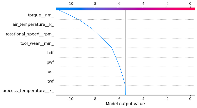
Image by author

Conclusion

SHAP values are a game-changer for machine learning interpretability. They empower us to move beyond black box models and gain valuable insights into how these powerful tools are working. By understanding the “why” behind model predictions, we can build more trust, improve our models, and ultimately make better decisions. So, dive in, explore the Shap package, and start unlocking the secrets of your machine learning models!

If you found value in this post, feel free to treat me to my favorite coffee, a cappuccino! 😊

If you found this post helpful, a clap would mean a lot. Don’t forget to follow me on Medium for more articles like this!

Data Science
Programming
Python
Machine Learning
Data
Recommended from ReadMedium