SGDClassifier: Untaught Lessons You Need to Know

A Deep Dive into the Hidden Secrets of the Linear Classifier

I recently published an article discussing the overlooked aspects of SGDRegressor, and in this piece, I delve into SGDClassifier. While some may assume that the two are simply variations of the same model for regression (continuous output) and classification (binary output), similar to KNeighborsRegressor vs. KNeighborsClassifier, or DecisionTreeClassifier vs. DecisionTreeRegressor, this article reveals the surprising ways in which they are linked.

I won’t rehash the topics already covered in the SGDRegressor article, such as the confusing name (SGD is instead a fitting algorithm than a machine learning model) and the comparison of Stochastic Gradient Descent (SGD) vs Gradient Descent. However, we will cover the loss functions used in SGDClassifier and the specific models with specific sets of hyperparameters.

We will delve into the peculiar connection between the linear regressor and linear classifier, focusing on their respective loss functions and the construction of a linear classifier. Furthermore, we will take a closer look at the different outputs produced by the linear classifier to gain a more comprehensive insight into its mechanism.

1. The Usually Taught Lesson

1.1 Linear Classifier using SGD

SGDClassifier is a classification algorithm used in machine learning that belongs to the family of linear models. The fitting algorithm Stochastic Gradient Descent (SGD) finds the optimal coefficients of the linear classifiers by updating the model’s parameters using the gradient of the loss function. The algorithm is beneficial for handling large-scale datasets, as it updates the model parameters on samples of observations rather than using the entire dataset, which can be computationally expensive.

1.2 SGDRegressor vs. SGDClassifier

Both SGDRegressor and SGDClassifier are linear models (and they are accordingly in the `linear_model` module) and use the same underlying fitting algorithm, namely SGD — Stochastic Gradient Descent. However, they differ in their specific applications.

The difference is that SGDRegressor is used for regression problems, where the goal is to predict a continuous output variable. On the other hand, SGDClassifier is used for classification problems, where the goal is to predict a categorical output variable.

As a result, the loss functions employed by the two models differ accordingly.

1.3 The Usual Loss Functions and the Hidden Models

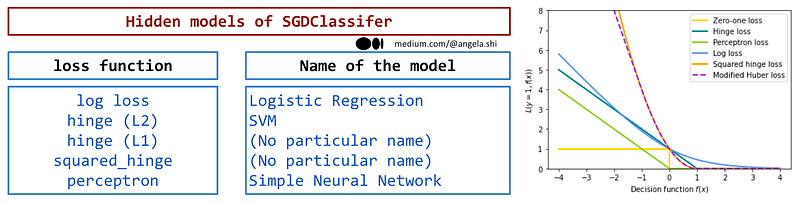
Similarly to SGDRegressor, conventional statistical models with specific names can be associated with certain loss functions in SGDClassifier.

• The use of log loss in a linear classifier leads to logistic regression. It’s worth noting that even if the coefficients of a logistic regression are penalized, it’s still considered a logistic regression model. This can be observed in implementing the estimator LogisticRegression in scikit learn, where there is an option to include a penalty term.
• The hinge loss function and L2 regularization in the cost function is used to obtain SVM. This model is often referred to as a soft-margin maximizer, where the maximization process is equivalent to minimizing the L2-norm of the coefficients. The name SVM primarily refers to using only a few observations, called support vectors, to define the model when trained using the dual form. However, when trained using the SGDClassifier, the model is trained in the primal form using stochastic gradient descent.
• There is no specific name for combining hinge loss with L1 penalty.
• The Perceptron loss used in a model can be viewed as a primary neural network, as established by researchers in the past. Further information on this topic can be found in this Wikipedia article on the perceptron.

There is a discussion about whether logistic regression is more of a regressor or a classifier. While some insights are available to shed light on this topic, I will provide a more comprehensive analysis in an upcoming article, exploring the issue from various perspectives.

2. The Unusual Relationship between Linear Classifier and Linear Regressor

2.1 The usual Relationship of Classifier vs. Regressor

Here is an illustration that displays the classifiers and regressors offered by scikit-learn. In the conventional supervised machine learning framework, there are two primary types of models: classifiers and regressors. These models operate differently based on the nature of the target variable they are designed to predict.

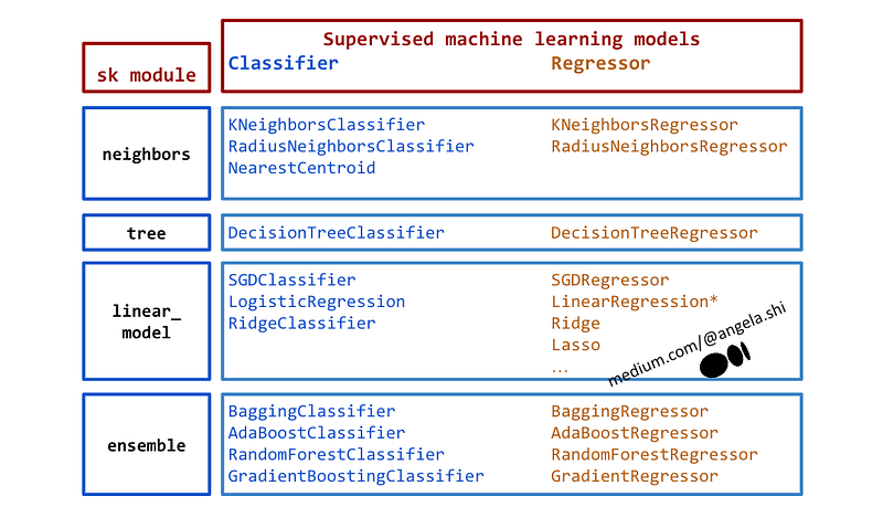
In scikit-learn’s neighbors module, the KNeighborsClassifier and KNeighborsRegressor are examples of distance-based estimators. These models use the distance between observations to identify the K nearest neighbours. For classification, the proportion of one class among the K nearest neighbours is used to calculate the probability of the observation belonging to that class. For regression, the prediction is the average value of the target variable among the K nearest neighbours.

In decision tree models, the DecisionTreeClassifier typically uses gini or entropy to determine the splits, while the DecisionTreeRegressor typically measures the reduction of variance to make the splits.

Now, what happens for the linear classifier and linear regressor? The normal relationship should be: they use distinct loss functions. However, you might be surprised to learn that there is more to this than meets the eye…

2.2 The Inclusion Relationship of Loss Functions

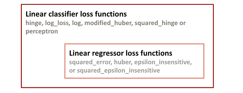
The scikit-learn documentation for SGDClassifier lists possible loss functions: hinge, log_loss, log, modified_huber, squared_hinge, perceptron, squared_error, huber, epsilon_insensitive, or squared_epsilon_insensitive. The documentation also includes this comment below:

‘squared_error’, ‘huber’, ‘epsilon_insensitive’ and ‘squared_epsilon_insensitive’ are designed for regression but can be useful in classification as well

So contrary to other estimators (KNeighbors or DecisionTree), there is something unusual between the two types of learning: all the loss functions for linear regressors can be used for the classification task.

Mathematically, there is no concept of a categorical variable in a function. The function only operates on numbers. To represent a categorical variable in a function, we often use binary indicators such as 0 and 1 or -1 and 1. However, these binary indicators are still numbers, so they are continuous. Therefore, the loss functions used in linear regression models, designed to handle continuous variables, can also be applied to categorical variables.

The use of loss functions designed for regressors in the SGDClassifier demonstrates that the distinction between regressors and classifiers is determined by the nature of the target variable in the training dataset rather than being an inherent characteristic of the model itself. Therefore, machine learning models are not inherently regressors or classifiers per se.

If the target variable in the training dataset is binary and the squared error is used, then it can be argued that linear regression or OLS regression is a classifier!

2.3 Linear Classifiers Do Not Exist in the first place

Let's take a closer look at the mathematical representation of the linear classifier model, y = wX + b. We can observe that it is identical to the one used in the linear regressor model. Therefore, the linear classifier and the linear regressor are essentially the same models, differing only in how the coefficients w and b are determined using various loss functions.

When the model y = wX + b is trained, this model will produce continuous values because w and b are continuous, and X contains numerical values.

Looking at it this way, when using the linear model, we solely perform regression because the output variable y is continuous. Well, at least, it is the case in the first place.

A linear classifier arises only when a threshold is defined for y. This is why -1 and 1 are usually selected as the two possible values for y in the training dataset. The sign of the output score determines the predicted class: if the score is positive, the predicted class is a positive class, and if it is negative, the predicted class is the negative class. And the model y = w X + b is an intermediate result to achieve binary classification. So it is called the decision function.

It should be noted that a linear classifier is initially designed to perform binary classification exclusively. However, we will discuss how it handles multiclass classification later in this article.

2.4 The Hyperplane Separator

After being trained on the training dataset with a loss function, the linear model y = wX + b can be used to predict classes. The hyperplane y = 0 functions as a linear separator for the space formed by X and y.

Using a hyperplane to separate data points based on their distance from the decision boundary applies not only to Support Vector Machine (SVM) but also to other linear classifiers such as logistic regression. Any linear classifier can be thought of as using a hyperplane to separate the data.

The hyperplane acts as a decision boundary, dividing the feature space into two regions: one region for each class.

From this viewpoint, the linear classifier can be considered a distance-based model because it measures the distance between a new observation and the hyperplane separator. This distance is used to make predictions about the class label of the new observation. This distance is proportional to the values given by the decision function.

3. Deep dive on Outputs of Linear Classifiers

Let’s investigate how the linear classifier functions by analyzing its outputs.

3.1 Outputs of the Linear Classifier

When dealing with a valid categorical variable, it is clear what each category represents, and calculating the proportion of one class among others is straightforward. However, for a linear classifier, the model being a mathematical function, additional intermediate outputs are involved in determining the final prediction. Let’s take a moment to recap these different kinds of outputs:

• Binary real output: The target variable in the training dataset typically consists of two categories, usually represented as 0 and 1. However, one may also use other values, such as -1 and 1, or even arbitrary values, such as 4 and 5. While there are no theoretical restrictions on the specific values used for binary classification, ensuring that only two categories are present is essential. However, conventionally, these values are transformed into -1 and 1, simplifying the equation and allowing us to refer to the positive and negative classes. In multi-class classification, the target variable can take on multiple values, each representing a different category. We will explore this topic further later in this section.
• Decision function value: The output of a linear model is a continuous value represented by the equation y = wX + b. While this is only an intermediary result, it is essential to keep it in mind as it is used in the loss functions to train the model.
• Binary predicted output: After computing the decision function value of a linear model, we can determine the expected class. If the value of y is greater than 0, the predicted class is 1. This final prediction of a classification task gives the linear classifier its name.
• Probability calculation: In a classification problem, assigning a probability to the predicted class is common to measure the confidence of the model’s prediction. While calculating probabilities is simple for distance and tree-based models, it can be challenging for linear classifiers, except for the logistic regression, which uses the log loss function. We will delve into this topic in the following section.

You may observe that the outputs are arranged in the order of the calculation based on the modelling perspective of SGDClassifier.

3.2 Probability calculation for a linear classifier

Once the linear model y = w X + b has been fitted, the next step is to calculate the probability of each prediction. There are two possible approaches:

The first approach consists of applying the logistic function to the decision function. The logistic function is used to convert the linear output of the classifier into a probability value between 0 and 1. The logistic function is defined as:

p = 1 / (1 + exp(-y))

where p is the probability value, and y is the linear output, aka the decision function value of the classifier.

The logistic function ensures that the predicted probability value is always between 0 and 1, regardless of the linear output value. If the linear output of the classifier is positive, the probability value will be greater than 0.5, indicating an optimistic class prediction. Conversely, if the linear output is negative, the probability value will be less than 0.5, indicating a pessimistic class prediction.

A noteworthy point from a statistical perspective is that logistic regression can be regarded as a regressor for probability. This is because the fitting process involves transforming the linear relationship between the input features and the output variable using the logistic function. Conceptually, the probability is first calculated, and then the maximum likelihood of all observations in the training dataset is optimized during the training process. To summarize, the outputs are modelled in a different order from the statistical perspective, but the optimization theory underlying them is fundamentally equivalent.

Isotonic regression is another method used to estimate probability values for a linear classifier. It is a non-parametric regression technique that estimates a non-decreasing function that maps the linear output of the classifier to the predicted probability values. Isotonic regression is useful when the linear output and probability values relationship is non-monotonic or has local minima/maxima.

The predicted probability values are estimated in isotonic regression by fitting a non-decreasing function to the training data. The estimated function is then used to predict the probability values for new observations based on their linear output.

3.3 Multiclass classification

To handle multiclass classification, distance-based classifiers and tree-based classifiers treat the output as a categorical variable and calculate the probability of each class based on its proportion among the other classes. Therefore, the calculation remains the same, regardless of the number of classes.

However, this is impossible with a linear classifier, which can only handle binary classification initially. While the SGDClassifier allows inputting the target variable with multiple classes, it uses a one-vs-one or one-vs-rest approach, training multiple binary classifiers, one for each class, and combining their predictions to make a final classification. This means that the original linear classifier model cannot handle multiclass classification intrinsically.

Alternatively, a mathematical-based function such as the softmax classification can be used for multiclass classification.

Conclusion

Like SGDRegressor, SGDClassifier incorporates classic models such as logistic regression and SVM. Although their names suggest a statistical origin, they can find a unified framework in machine learning through SGDClassifier.

The linear classifier has an unusual relationship with the linear regressor regarding loss functions. By examining its various outputs, we better understand how it operates. We have also discussed the limitations of linear classifiers in handling multiclass classification tasks and the different strategies used to overcome these limitations, such as one-vs-one and one-vs-rest approaches.