Serving ML models at scale using Mlflow on Kubernetes

Part 1 — How to deploy Mlflow tracking instance on Kubernetes?

TLDR

MLflow is a commonly used tool for machine learning experiments tracking, models versioning, and serving. In our first article of the series “Serving ML models at scale”, we explain how to deploy the tracking instance on Kubernetes and use it to log experiments and store models.

Introduction

Mlflow is a widely used tool in the data science/ML community to track experiments and manage machine learning models at different stages. Using it, we can store metrics, models, and artifacts to easily compare models’ performances and handle their life cycles. Besides, Mlflow provides a module to serve models as an API endpoint which facilitates their integration to any product or web app.

That being said, using machine learning in products online is cool, but depending on model size, nature (ML, deep learning,… ), and load (users’ requests) it could be challenging to dimension the needed resources and guarantee a reasonable response time. Therefore, using a scalable infrastructure such as Kubernetes clusters is key to maintain service availability and performance in the inference phase.

In this context, we are publishing a three-article series in which we answer the following questions:

- How to deploy and use Mlflow tracking instance on Kubernetes? - How to serve Machine learning models as API using Mlflow? - How to handle a high number of requests and make our inference task scalable for industrialized products?

So let’s start this first article by introducing Kubernetes and its components and go through the deployment of a tracking instance to log models.

Overview on Kubernetes

Kubernetes is an open-source project, released by Google in 2014. It is a container control and orchestration system that allows automatic applications deployment, scaling, and scheduling. It has the following architecture:

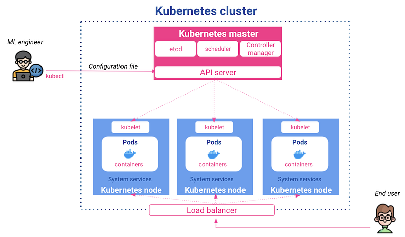
Master: It handles input configurations, schedules containerized apps on the different nodes, and monitors their states. The master is composed of:

• API server: allows the interaction with the cluster and validates the commands sent by the developer to update the cluster or the app state.
• Scheduler: decides on which nodes new objects should be run to ensure stability and load balancing.
• Etcd: a key-value database that stores the different resource configurations and states
• Controller Manager: monitors the cluster state and the different resources and makes sure that the current state matches the desired one.

Nodes: they are the execution nodes in which deployed containers live. Their main components are:

• Pods: are the basic fundamental execution unit in Kubernetes. A Pod encapsulates an application either as a single container or multiple containers that work together with shared storage volumes and networks.
• Kubelet: is an agent for inspecting the container status and communicating with the Kubernetes master.

It’s the go-to choice when an application has multiple services communicating with each other as it ensures that every service has its own containerized environment with a set of rules to interact with others. Besides, it offers the interesting capability to scale up an application without worrying about managing or synchronizing new services and to balance resources between different machines.

From a high-level perspective, as data scientists or ML engineers, we will interact with Kubernetes via its server API using CLI commands or YAML config files either to deploy and expose apps or get our resources states.

Hands-on pre-requirements

For this hands-on, we will use GCP as a cloud provider. First, we need to :

1. Create the infrastructural elements

• mlflow_gke: a bucket to store files, datasets…
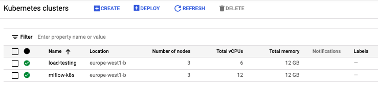
• mlflow-k8s: a three-node (e2-highcpu-4) GKE cluster to deploy both the tracking module and the machine learning model.
• load-testing: a three-node (e2-standard-2) GKE cluster to perform load tests. It will be used in the third article of this series.

2. Configure the local workstation

• Install python requirements to interact with GCP and mlflow cli

pip install mlflow gcsfs google-cloud google-cloud-storage kubernetes

• Have gcloud and kubectl configured with the credentials to access the GCP project and the clusters
• Have the Helm CLI installed and initialized. Please find here the instructions in case you don’t have the client yet.

3. Clone the hands-on project repository to get the code

git clone https://github.com/artefactory/mlflow-serving-example

Mlflow Tracking instance deployment

1. Setup the Cluster environment

• Create a service account to allow the interaction with GCS This could be done via the google cloud console, under the iam section. We need to create a service account with storage object admin permission, generate an authentication key, and download it as keyfile.json
• Mount the authentication file as a secret Secrets allow us to handle in a secure way the credentials so that they are visible only to relevant resources. For this, we will create a secret volume and expose the authentication file only to the needed containers.

kubectl create secret generic gcsfs-creds --from-file=./keyfile.json

2. Tracking server deployment

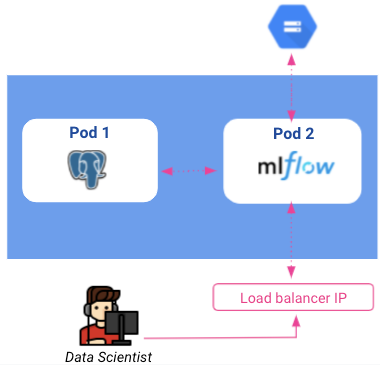
• Postgres store Postgre serves as a backend storage element for mlflow to save models metadata and metrics. To deploy it we will use Helm: a resources manager for Kubernetes where many applications are available in the format of charts or templates that could be configured with simple commands.

#docs: https://artifacthub.io/packages/helm/bitnami/postgresql

helm repo add bitnami https://charts.bitnami.com/bitnami

helm install mlf-db bitnami/postgresql --set postgresqlDatabase=mlflow_db --set postgresqlPassword=mlflow --set service.type=NodePort

• Tracking instance We will also use Helm charts to deploy the tracking server, but first, we need to build a docker image with the version we want so that it could be downloaded and deployed by Helm. Notice that for Postgres, the image was already on a public repository, however here we will create our own image.

cd mlflow-serving-example

docker build --tag ${GCR_REPO}/mlflow-tracking-server:v1 --file dockerfile_mlflow_tracking .

docker push ${GCR_REPO}/mlflow-tracking-server:v1

Once the image is pushed to the image registry we can deploy it on the cluster via helm using the below commands.

helm repo add mlflow-tracking https://artefactory.github.io/mlflow-tracking-server/

helm install mlf-ts mlflow-tracking/mlflow-tracking-server \
--set env.mlflowArtifactPath=${GS_ARTIFACT_PATH} \
--set env.mlflowDBAddr=mlf-db-postgresql \
--set env.mlflowUser=postgres \
--set env.mlflowPass=mlflow \
--set env.mlflowDBName=mlflow_db \
--set env.mlflowDBPort=5432 \
--set service.type=LoadBalancer \
--set image.repository=${GCR_REPO}/mlflow-tracking-server \
--set image.tag=v1

Now, Mlflow should be up and running and the UI should be accessible via the load balancer IP. We can check the assigned IP using kubectl get services. Also, we can debug the deployment by accessing logs via kubectl describe pods. So far, our current architecture looks like the following:

Please note that load balancers are accessible to anyone on the internet, so it is essential to think about securing our tracking instance by adding an authentication layer. This could be done with the identity-aware proxy on GCP but won’t be tackled in this article.

3. Basic model creation

Now that our infrastructure and Mlflow instance are ready, we can try to run a simple ML model and save it in the model registry for later use.

We will be using the wine-quality dataset which is composed of around 4900 samples and 11 features reflecting wine characteristics. The label ranges from 3 to 9 and could be seen as ratings.

This is a classic example, in which we train an Xgboost regression model and store it along with its parameters and metrics. The full code could be found in this notebook.

You may have noticed that Mlflow integration is straightforward and it could be summarized in the below code snippet that invokes mlflow.start_run(), mlflow.log_param(), mlflow.log_metric() and mlflow.xgboost.log_model() to respectively create a new experiment, store the training parameters, the evaluation metrics and the trained model itself.

By running the provided notebook, a new row will be added in the tracking instance interface that corresponds to the new experiment.

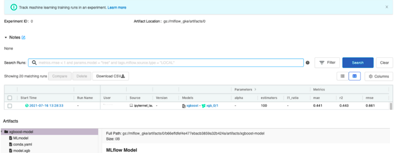
Finally, supposing that we are satisfied with the model performance, we can load it from the tracking instance and use it for inference in python. This could be done also with the notebook shared previously. Notice that in this example, we loaded the model using the run ID but keep in mind that Mlflow offers also other interesting ways to identify models by tags, versions, or stages. For more details please refer to the model registry documentation here.

Conclusion

Throughout this article, we managed to deploy Mlflow tracking instance to handle our data science experiments and we went through a quick example showing how to log a model and save it for future inference on python. In the next article of this series, we will learn how to serve this model as an API. This has great importance as it facilitates the interaction with the model and its integration into a product or an application. Moreover, doing it on Kubernetes ensures that it remains easily scalable and able to handle different load levels.