Sensitivity Analysis with SALib: A Powerful Data Analysis Tool

A mathematical function or neural network can be highly complex, so the relationships between the input and output are usually poorly understood. Sensitivity analysis studies the impacts of independent inputs on the output. We could observe which features are influential by measuring the changes in the output with varying values of different inputs. If the sensitivities of the basic inputs can be analysed, more insights can be revealed to stakeholders to make decisions. For example, when building financial models, sensitivity analysis can provide insights such as how much the revenue increase if the customer traffic increase, how about decreasing the price, and which input is more impactful?

1. Sensitivity Analysis Approaches

(1) Local Approach

This approach is more intuitive. We could select a base, for example, the mean of one feature input. Then we increase 5% of this input,fixing other inputs and check how much the output changes. It’s called Local Approach because the evaluation is based on this initial point, if the function/model is non-linear, it could not capture the global sensitivity. This naive calculation is called One-at-a-time(OAT) method, evaluate one feature at a time. An extension to OAT is Morris algorithm. In Morris, OAT is randomized, the OATs are initialised from many points and then calculate the mean and variance of all OATs. larger mean indicates higher impact, higher variance reflects the non-linearity.

Local approaches cost less computation, but they do not analyse the interaction among the input features.

(2) Global Approach

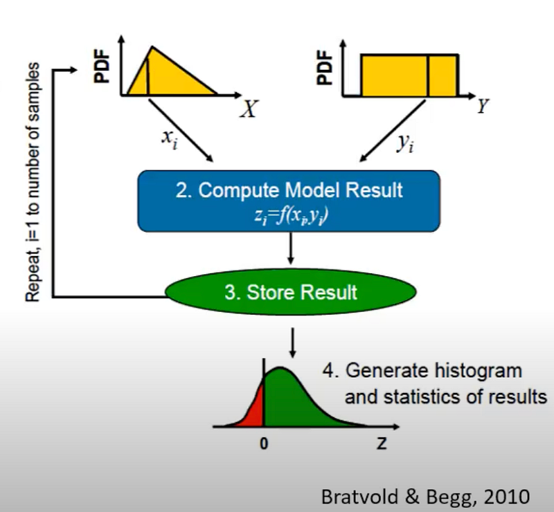
Global approaches, on the other hand, consider input distributions and stochastic responses. Therefore, it’s more suitable for high-dimensional and non-linear functions.

There are four main groups of algorithms, according to [1]:

(1) Variance-based

(2) Reginonal SA

(3) Linear Model

(4) Tree-based

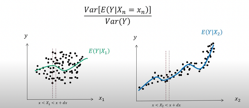
Sobol, which is avariance-based algorithm, might be the most classical one. It calculates how much the variance of input can impact the variance of output.

Hoeffding decomposition [3] states that the variance of the output can be uniquely decomposed into summands of increasing dimensions under orthogonality constraints.

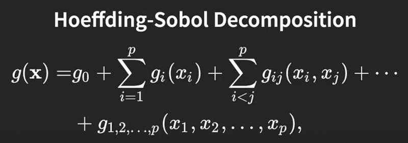
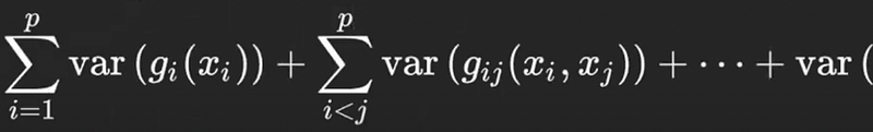
Following this direction, Sobol[4] introduces variability measures, which is called Sobol sensitivity indices. The first order indices, which is the first term below, calculating the impact of a single input. The second order indices(the second term below), consider two inputs, as a result, it consider the interactions. And the last term consider all inputs.

You can check the online course[1] for more global sensitivity analysis theories.

2. SALib — A Python Sensitivity Analysis Library

Since sensitivity analysis is important, there are already many libraries implementing the algorithms mentioned above, such as SobolGSA in C#, MATLAB, and Python, UQLab in MATLAB, SALib (Herman and Usher, 2017) in Python, MADS.jl in Julia. SALib is what I choose to use. https://github.com/SALib/SALib

This video tutorial introduces the library: https://www.youtube.com/watch?v=gkR_lz5OptU&t=204s

It’s quite easy to use, there are 4 steps.

(1) Define the model inputs (the range of the inputs, e.g. -10 to 10 is [10,10])

(2) Generate samples (since we use monte carlo)

(3) Use your model to calculate the output

(4) Select different implemented algorithm to analyse

3. Analysis Example

Here is a simple example from the official documentation, using Sobol to quantify the sensitivities of input parameters in Ishigami Function.

(1) Ishigami Function

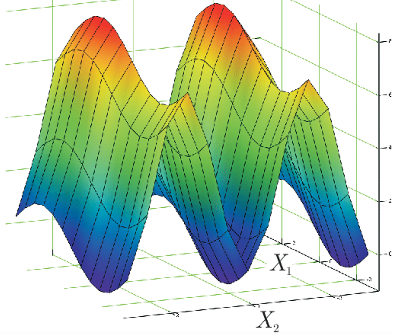
This function is often used to benchmark the performance of different global sensitivity analysis methods. Let a=7 and b=0.1 (Crestaux et al. (2007) and Marrel et al. (2009)). The function is

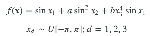
It is hard to tell which input is the most impactful one, especially between x1 and x2. There is also colleration/interaction between x1 and x3, which will also be captured by global sensitivity analysis.

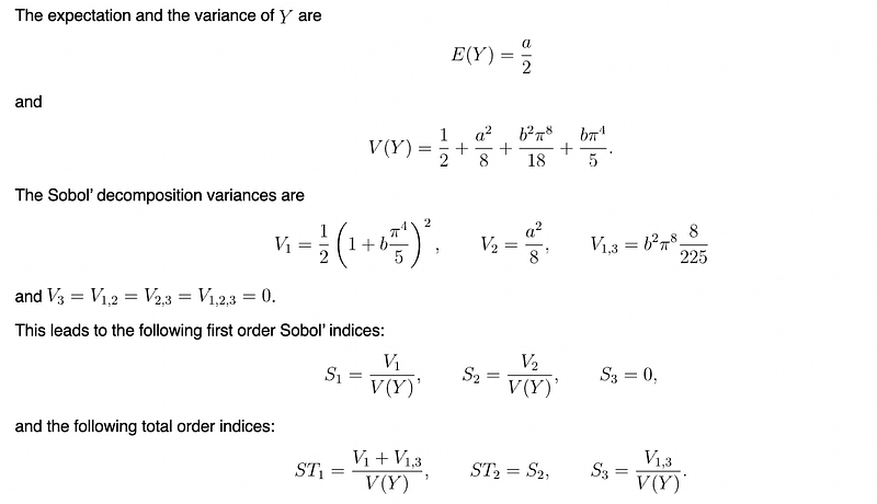
We know the ground-truth value of sobol indices, then we can use SALib to calculate it.

(2) Using SALib to analyse

see doc here : https://salib.readthedocs.io/en/latest/getting-started.html

The result is [ 0.31683154 0.44376306 0.01220312],which means x2 is the most impactful one, and x3 is the least influential one(it is 0 actually)

from SALib.sample import saltelli
from SALib.analyze import sobol
from SALib.test_functions import Ishigami
import numpy as np

# Define the model inputs
problem = {
    'num_vars': 3,
    'names': ['x1', 'x2', 'x3'],
    'bounds': [[-3.14159265359, 3.14159265359],
               [-3.14159265359, 3.14159265359],
               [-3.14159265359, 3.14159265359]]
}

# Generate samples
param_values = saltelli.sample(problem, 1024)

# Run model (example)
Y = Ishigami.evaluate(param_values)

# Perform analysis
Si = sobol.analyze(problem, Y, print_to_console=True)

# Print the first-order sensitivity indices
print(Si['S1'])

-------------------------------------------------------------------

[ 0.31683154 0.44376306 0.01220312]

References:

[1]Jef Caers, Stanford Gs260:

https://www.youtube.com/watch?v=P8Rfipkid3w&t=4s

and https://www.youtube.com/watch?v=vBuWB9WuFhA&t=1603s

[2] ML and the Physical World 2020: Lecture 9 Sensitivity Analysis

https://www.youtube.com/watch?v=I5ZlCLR89AU

[3]Hoeffding, W. (1992). A class of statistics with asymptotically normal distribution. In Breakthroughs in statistics (pp. 308–334). Springer, New York, NY.

[4] Sobol’, I. Y. M. (1990). On sensitivity estimation for nonlinear mathematical models. Matematicheskoe modelirovanie, 2(1), 112–118.

[5] Will Usher: Using the SALib library for conducting sensitivity analyses of models https://www.youtube.com/watch?v=gkR_lz5OptU&t=204s

[6] Global Sensitivity Analysis (n Fall 2020 and Spring 2021, this was MIT’s 18.337J/6.338J: Parallel Computing and Scientific Machine Learning course. )https://www.youtube.com/watch?v=wzTpoINJyBQ&t=386s

[7] SALib Documentation : https://buildmedia.readthedocs.org/media/pdf/salib/stable/salib.pdf