Summary

Scikit-plot is a Python library that simplifies the visualization of machine learning models by providing straightforward and easy-to-understand functions for evaluating and displaying various aspects of model performance and structure.

Abstract

Scikit-plot is designed to enhance the visualization capabilities for machine learning models built using scikit-learn. It offers a range of intuitive plotting functions that facilitate the visualization of evaluation metrics such as confusion matrices, ROC curves, KS statistics, precision-recall curves, and silhouette analysis for clustering. The library also supports model visualization through learning curves, feature importance plots, elbow plots for clustering, and variance and 2D projection plots for dimensionality reduction with PCA. These functionalities are aimed at making the process of model interpretation and diagnosis more accessible and efficient for data scientists and machine learning practitioners. The article emphasizes the ease of use and the direct applicability of scikit-plot's functions, while also noting that some advanced features may require users to consult the library's documentation for a deeper understanding.

Opinions

The author suggests that scikit-plot is user-friendly and enhances the interpretability of machine learning models.
Visualizations provided by scikit-plot are considered straightforward and easy to understand, which can be beneficial for both beginners and experienced practitioners.
The article implies that scikit-plot integrates seamlessly with scikit-learn and Matplotlib, leveraging the strengths of both libraries.
It is acknowledged that while most functions are simple to use, some may have advanced features that necessitate further exploration of the scikit-plot documentation.
The author expresses that using scikit-plot in machine learning projects can make modeling more efficient and enjoyable.

Scikit-plot Making Machine Learning Model Visualization Easier

scikit-learn (sklearn) is a common machine learning library in the Python environment, containing popular classification, regression, and clustering algorithms. After training a model, it is common to visualize the model, requiring the use of Matplotlib for display.

scikit-plot is a library based on sklearn and Matplotlib, primarily designed for visualizing well-trained models, with straightforward and easy-to-understand functionalities.

pip install scikit-plot

Visualization of Evaluation Metrics

scikitplot.metrics.plot_confusion_matrix quickly displays the confusion matrix, showcasing the model’s prediction results and the labels calculated.

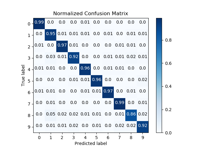
import scikitplot as skplt

rf = RandomForestClassifier()
rf = rf.fit(X_train, y_train)
y_pred = rf.predict(X_test)

skplt.metrics.plot_confusion_matrix(y_test, y_pred, normalize=True)
plt.show()

scikitplot.metrics.plot_roc quickly displays the ROC curves for each class predicted by the model.

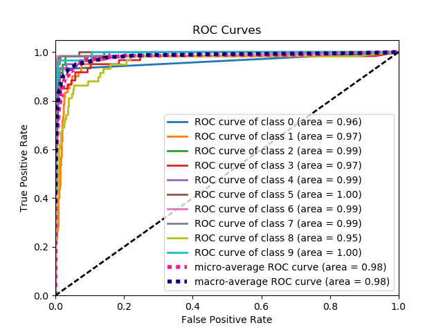
import scikitplot as skplt

nb = GaussianNB()
nb = nb.fit(X_train, y_train)
y_probas = nb.predict_proba(X_test)

skplt.metrics.plot_roc(y_test, y_probas)
plt.show()

scikitplot.metrics.plot_ks_statistic generates the KS statistic plot from labels and scores/probabilities.

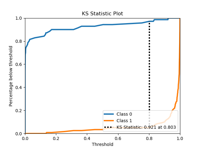
import scikitplot as skplt

lr = LogisticRegression()
lr = lr.fit(X_train, y_train)
y_probas = lr.predict_proba(X_test)

skplt.metrics.plot_ks_statistic(y_test, y_probas)
plt.show()

scikitplot.metrics.plot_precision_recall generates precision-recall curves from labels and probabilities.

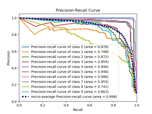
import scikitplot as skplt

nb = GaussianNB()
nb.fit(X_train, y_train)
y_probas = nb.predict_proba(X_test)

skplt.metrics.plot_precision_recall(y_test, y_probas)
plt.show()

scikitplot.metrics.plot_silhouette performs silhouette analysis on clustering results.

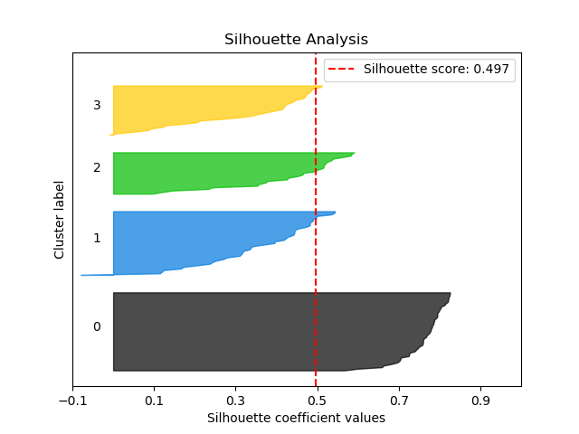
import scikitplot as skplt

kmeans = KMeans(n_clusters=4, random_state=1)
cluster_labels = kmeans.fit_predict(X)

skplt.metrics.plot_silhouette(X, cluster_labels)
plt.show()

scikitplot.metrics.plot_calibration_curve plots the calibration curve of a classifier.

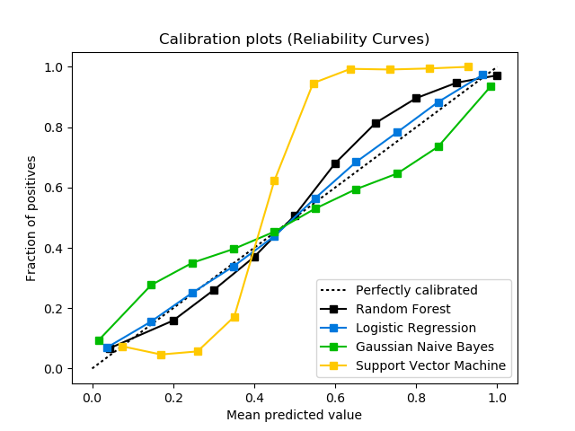
import scikitplot as skplt

rf = RandomForestClassifier()
lr = LogisticRegression()
nb = GaussianNB()
svm = LinearSVC()
rf_probas = rf.fit(X_train, y_train).predict_proba(X_test)
lr_probas = lr.fit(X_train, y_train).predict_proba(X_test)
nb_probas = nb.fit(X_train, y_train).predict_proba(X_test)
svm_scores = svm.fit(X_train, y_train).decision_function(X_test)
probas_list = [rf_probas, lr_probas, nb_probas, svm_scores]
clf_names = ['Random Forest', 'Logistic Regression',
              'Gaussian Naive Bayes', 'Support Vector Machine']

skplt.metrics.plot_calibration_curve(y_test,probas_list,clf_names)
plt.show()

Model Visualization

scikitplot.estimators.plot_learning_curve generates training and testing learning curves under different training samples.

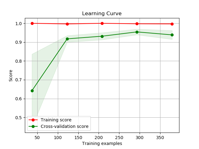
import scikitplot as skplt

rf = RandomForestClassifier()
skplt.estimators.plot_learning_curve(rf, X, y)
plt.show()

scikitplot.estimators.plot_feature_importances visualizes feature importances.

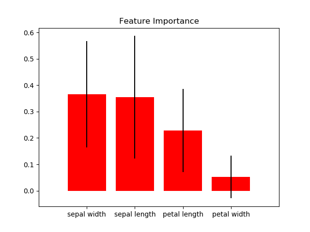
import scikitplot as skplt

rf = RandomForestClassifier()
rf.fit(X, y)

skplt.estimators.plot_feature_importances(
     rf, feature_names=['petal length', 'petal width',
                        'sepal length', 'sepal width'])
plt.show()

Clustering Visualization

scikitplot.cluster.plot_elbow_curve displays the elbow plot for clustering.

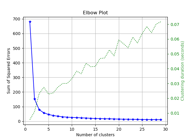
import scikitplot as skplt
kmeans = KMeans(random_state=1)

skplt.cluster.plot_elbow_curve(kmeans, cluster_ranges=range(1, 30))
plt.show()

Dimensionality Reduction Visualization

scikitplot.decomposition.plot_pca_component_variance plots the explained variance ratio of PCA components.

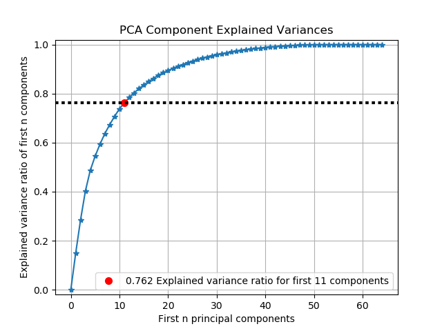
import scikitplot as skplt
pca = PCA(random_state=1)
pca.fit(X)

skplt.decomposition.plot_pca_component_variance(pca)
plt.show()

scikitplot.decomposition.plot_pca_2d_projection plots a scatter graph after PCA dimensionality reduction.

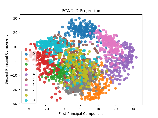
import scikitplot as skplt

pca = PCA(random_state=1)
pca.fit(X)

skplt.decomposition.plot_pca_2d_projection(pca, X, y)
plt.show()

In this post, we summarized 11 unique scikit-plot functions useful in your projects. Most of the functions are easy to use and straightforward, but some may have more advanced features that require further reading of scikit-plot documentation. Have a fun to use them in your projects for easier and efficient modelling.

Thanks for your reading.