Summary

The article discusses the use of the Random Forest classifier in Google Earth Engine for generating a forest/non-forest (FNF) map using PALSAR-2 SAR imagery, including pre-processing steps like speckle filtering, and the incorporation of additional bands such as elevation and slope for improved classification accuracy.

Abstract

The article, part of a series on SAR forest monitoring, details the process of performing a supervised classification to create an FNF map using PALSAR-2 data within Google Earth Engine. It emphasizes the advantages of custom FNF map generation, such as enhanced accuracy, temporal consistency, and the ability to make regular updates. The author outlines the steps taken, including speckle filtering, acquisition of training data for three primary classes (forest, non-forest, and water), and the use of the Random Forest algorithm for classification. The article also explores the addition of elevation and slope bands from the ALOS World Digital Surface Model to improve classification results, demonstrated by a comparison of classified maps with and without these additional bands. Post-classification cleaning is discussed, along with potential improvements and considerations for error sources in SAR image classification. The importance of FNF maps for monitoring forest cover changes over time is highlighted, with an invitation for reader engagement on their use and preferred approaches.

Opinions

The author believes that generating a custom FNF map offers significant benefits over using pre-existing global land cover maps.
It is suggested that incorporating additional bands, such as elevation and slope, can substantially improve classification accuracy.
The author values the use of SAR imagery for forest monitoring due to its ability to penetrate clouds and its independence from sunlight, which is particularly useful for tropical forest monitoring.
There is an emphasis on the importance of understanding topography and implementing terrain correction techniques, especially in mountainous regions.
The author acknowledges that the true accuracy of the classifier can only be assessed using an independent testing dataset, not just the training data.
The article encourages further research and experimentation with additional bands, model parameter tuning, and error source mitigation to enhance classification outcomes.

SAR Forest Monitoring Series Part3: PALSAR-2 Forest Non-forest Classification using Random Forest classifier in Google Earth Engine

To learn more about SAR remote sensing, please visit my series HERE.

Here, I discuss a basic supervised classification to generate a FNF map and some ideas to improve the classification. While several global land cover and forest/non-forest (FNF) maps are accessible through the Google Earth Engine (GEE) data catalog [1], such as the CORINE land cover map, Copernicus global land cover layer, ESA world cover, MODIS land cover type map, and the global PALSAR-2/PALSAR forest/non-forest map, there are distinct advantages to generating your own forest/non-forest map. Customization, accuracy enhancement, temporal consistency, and regular updates are among the key benefits that can be achieved through this approach.

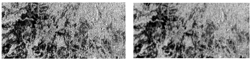
In the preceding segments of the series (PART1 and PART2), we covered accessing PALSAR-2 imagery in GEE, visualizing the data, and gaining insights into the backscatter properties. In this installment, we proceed directly to the classification process, incorporating one additional step in the pre-processing of PALSAR-2 imagery — Speckle filtering. For this purpose, a basic smoothing filter with a radius of 50 is applied, although it’s important to note that this may result in reduced image resolution. Notice that in figure(1) the salt and pepper effect in the SAR image is reduced upon filtering (right image).

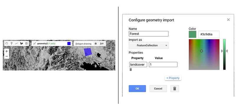
Figure (1): PALSAR-2 image before (left) and after(right) speckle filtering

As this is a supervised classification approach, the acquisition of training data is imperative to effectively train the classifier. Three primary classes are considered: Forest, non-forest, and water. To gather reference data, various sources can be utilized, including in-situ measurements, high-resolution optical imagery, or existing land cover maps. In this instance, I have used the knowledge of SAR backscatter properties together with the available PALSAR-2 global FNF map — HERE. Understanding that darker areas in SAR imagery typically represent bare land, water, or unvegetated regions, while brighter areas often indicate forests or settlements, we use this knowledge in conjunction with the existing map to delineate training samples. To accomplish this, one can navigate to the geometry tool, draw polygons directly onto the image, access geometry properties, and assign the corresponding class name. Additionally, an extra property name can be designated, with the class value specified accordingly as shown in figure (2). Following this process, import the geometry as a feature collection, with the option to customize the color scheme if desired.

Figure (2): Collecting training samples for classification

Now that all three classes have been imported into GEE as feature collections with class values 1 (forest), 2 (non-forest), and 3 (water), the next step involves merging these feature collections. Following this, define the bands necessary to train the data, proceed to train the classifier, and initiate the classification process.

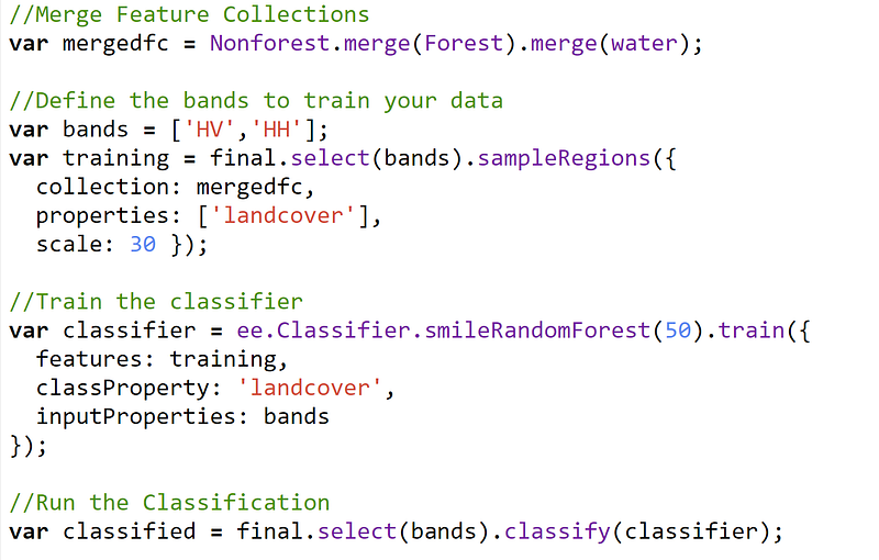
Random forest algorithm creates a set of decision trees from a sample of training data. It builds a committee of a number of individual decision tree classifiers and the votes cast by each tree are later combined to make a decision based on the majority votes derived. It takes a random set of 2/3 of training samples to build the decision trees and uses the remaining 1/3 of the sample to estimate error and importance of predictor variables. The number of trees I have used here is 50 — you can tweak it and experiment to see changes in classification.

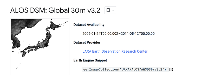
I wanted to improve the classification further and decided to include more bands. I added the slope and elevation bands from the ALOS World Digital Surface Model elevation (DSM) to the existing SAR bands and trained the classifier using the new bands. Read more about the DSM HERE.

I trained the classifier again with the bands — HH, HV, elevation and slope and the results surprised me! Before I show the comparison between the results, I want to mention that I created a confusion matrix. But this was based on the training data and hence it is not a true representation of accuracy. You need to create an independent dataset or a new testing set of polygons and run the confusion matrix on it to check the true accuracy of the classifier!

Results

The comparison depicted in figure (3) illustrates the differences between classified maps generated by running the classification solely on the SAR bands (HH and HV) versus incorporating additional variables such as elevation and slope.

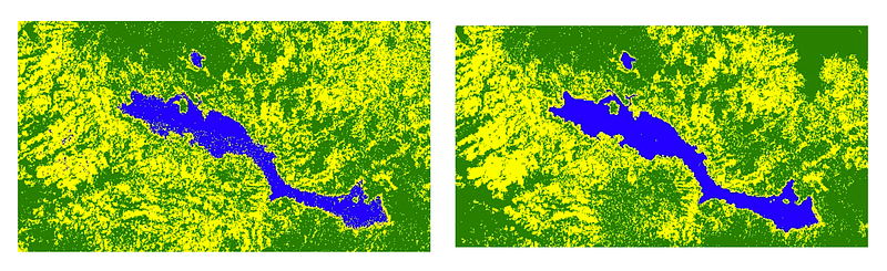
Figure (3): Classification only on SAR bands(left), classification with all 4 bands(right)

Clearly, you can see the difference. More the bands, better the classification. A random forest variable importance plot gives a better understanding of the input variables that are important for the classification.

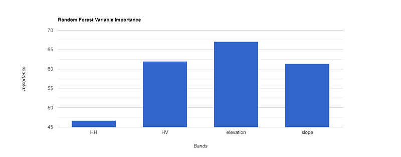
Notice that elevation is the most important variable followed by HV for this FNF classification!

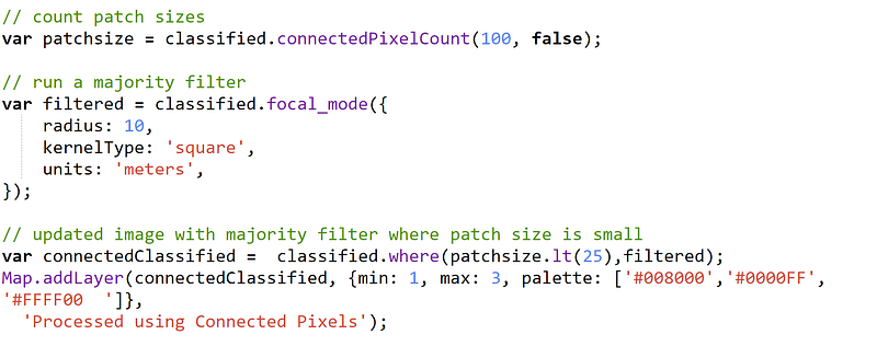
As a next step, post classification cleaning was performed by applying a majority filter as shown below.

Key notes: a few tips to improvise the classification further

Further improve the classification by adding more bands such as the Gray Level Co-occurrence Matrix texture measures extracted from the SAR images and SAR ratio images (HH/HV)
You can tune the RF model parameters and experiment with them. Read more in [2][3][4]
As mentioned before, create a new testing dataset and perform the accuracy assessment.
Understanding the topography of the study area is crucial. In mountainous regions, it becomes essential to implement terrain correction techniques.
Consider the possible error sources that can occur in a SAR image:
Error sources in SAR image classification include shadows, incidence angle variations, and moisture content. It’s advisable to check weather conditions since although SAR is generally not impacted by weather, errors can arise, especially when the ground is wet. Changes in the dielectric constant due to moisture content, and errors induced by freezing conditions, should also be considered.

FNF maps enable continuous monitoring of changes in forest cover over time. By comparing FNF maps from different time periods, researchers and policymakers can assess deforestation, reforestation, and forest degradation trends, helping guide conservation efforts and land management strategies.

Do let me know what you use the FNF maps for and what approaches you prefer! This will help us learn and grow together!

If you liked this article, then consider clapping for it! You also may want to follow me for more stories like this or subscribe to my email https://medium.com/@preet.balaji20/subscribe. Thank you for your support!

References

[1]https://developers.google.com/earth-engine/datasets/tags/landcover

[2] Gandhi, Ujaval, 2021. End-to-End Google Earth Engine Course. Spatial Thoughts. https://courses.spatialthoughts.com/end-to-end-gee.html

[3] Breiman, L., 2001. Random Forests. Mach. Learn. 45, 5–32. https://doi.org/10.1023/A:1010933404324

[4] Gislason, P.O., Benediktsson, J.A., Sveinsson, J.R., 2006b. Random Forests for land cover classification. Pattern Recognit. Lett., Pattern Recognition in Remote Sensing (PRRS 2004) 27, 294–300. https://doi.org/10.1016/j.patrec.2005.08.011