RSI divergence trading strategy

Looking for divergence between price and oscillator can be very helpful to enhance your basic strategy. But in this article, I would like to test RSI divergence as standalone trading strategy

What divergence in trading really is. Divergence has, a place when technical indicator (RSI in this case) -oscillator — doesn’t follow the price of instrument, in the sense that doesn’t reach new highs or lows when price does it. Divergence in technical analysis, can be very interesting strategy by itself, but in my opininon, it should be an addition to another strategy as complementary signal to make a trade. The best way to explain it, will be a graphical presentation.

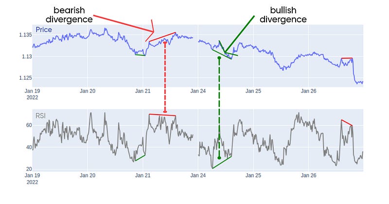
As you can see on the chart RSI doesn’t follow price of the instrument in marked points. Another important information, we can infer from the chart is, that a divergence is potential point of trend reversal. All of these let us to assume, that divergence can be a significant enhancement of every trading strategy, and of course can be standalone strategy.

How to find RSI divergence in Python ?

Now when we have theoretical background of that, what is a divergence in trading, let’s try to find some algorithm in Python, that let us find divergence on the chart. Oscillator (indicator), that will be used is RSI, but there are also another oscillators (MACD, Stochastic Oscillator), which can be compared to price chart, in order to find divergence. Ok, first task is to calculate RSI, and with talib library, it is very easy.

import pandas as pd
import numpy as np
import matplotlib.pyplot as plt
from scipy.signal import argrelextrema
import plotly.graph_objects as go
from plotly.subplots import make_subplots
import talib as ta
from scipy import stats



#import data
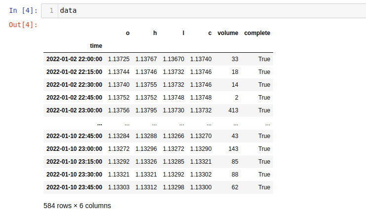
data_all=pd.read_csv('EUR_USD_2022_M15.csv', parse_dates=['time'], index_col='time')

#choose one month to better visualize 
data=data_all.loc['2022-01-02':'2022-01-10']


#calculate RSI

data['RSI']=ta.RSI(data['c'], 14)

As I said earlier, divergence is related to highs and lows of price and oscillator. So now we should find local minima and maxima. To obtain this I will use argrelextrema function from scipy.signal library.

def find_extrema(data, order, how='hh'):
    extremas=None
    
    if how=='hh':
        extremas=argrelextrema(data, comparator=np.greater, order=order)[0]
    if how=='ll':
        extremas=argrelextrema(data, comparator=np.less, order=order)[0]
    
    extremas_pairs=[extremas[i:i+2] for i in range(len(extremas))]
    return extremas_pairs

Code requires, a little bit of explanation, argrelextrema function especially. Function takes as arguments:

• data — values as array,
• comparator — if we are looking for highs, np.greater is the best choice, to find lows use np.less comparator,
• order — how many samples (points) should be used to comparison

In find_extrema function, data, order and which type of extrema we are looking for — higher highs (‘hh’) or lower lows (‘ll’) should be declared. Let’s see how function works.

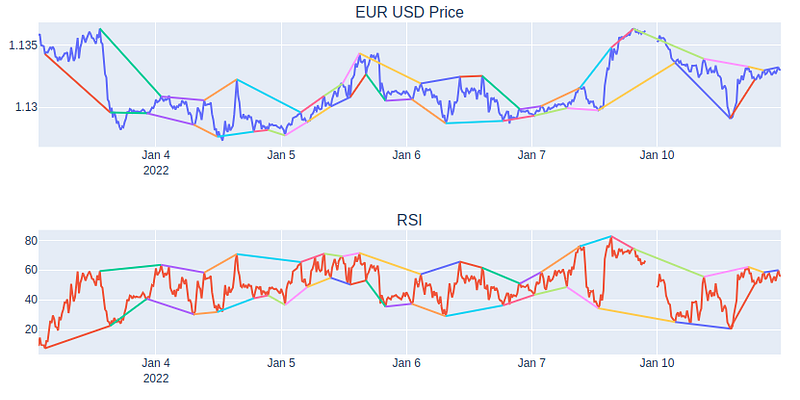
#find extremas for price
hh_price=find_extrema(data['c'].values, order=10, how='hh')
ll_price=find_extrema(data['c'].values, order=10, how='ll')

And let’s to visualize results.

fig=make_subplots(rows=2, cols=1, subplot_titles=("EUR USD Price", "RSI"))
fig.append_trace(go.Scatter(x=data.index, y=data['c'].values, mode='lines'), row=1,col=1)
fig.append_trace(go.Scatter(x=data.index, y=data['RSI'].values, mode='lines'), row=2,col=1)
for h_line in hh_price:
    fig.append_trace(go.Scatter(x=data.iloc[h_line].index, y=data['c'].iloc[h_line], mode='lines'), row=1, col=1)
for l_line in ll_price:
    fig.append_trace(go.Scatter(x=data.iloc[l_line].index, y=data['c'].iloc[l_line], mode='lines'), row=1, col=1)
for h_line_rsi in hh_price:
    fig.append_trace(go.Scatter(x=data.iloc[h_line_rsi].index, y=data['RSI'].iloc[h_line_rsi], mode='lines'), row=2, col=1)
for l_line_rsi in ll_price:
    fig.append_trace(go.Scatter(x=data.iloc[l_line_rsi].index, y=data['RSI'].iloc[l_line_rsi], mode='lines'), row=2, col=1)
fig.update_xaxes(rangebreaks=[dict(bounds=['sat', 'mon'])])
fig.show()

Local extremas are obtained. We can infer from the chart, that RSI oscillator strictly follow the price, so, if highs and lows of price are calculated, dates when they occurs reflect dates on the RSI chart. Next step is to filter, that lines which differ of their direction of slope. In this case useful will be function linregress from scipy.stats. This function calculate numerical features for the regression line, and one from this features is slope. The rules will be very simple, if sign of slope of the lines are different, it means that divergence occured.

def find_divergence(df, order):
    hh_pairs=find_extrema(df['c'].values,order, 'hh')
    ll_pairs=find_extrema(df['c'].values,order, 'll')
    
    bear_div=[]
    bull_div=[]
    
    for p in hh_pairs:
        
        x_price=p
        y_price=[df['c'].iloc[p[0]], df['c'].iloc[p[1]]]
        slope_price=stats.linregress(x_price, y_price).slope
        x_rsi=p
        y_rsi=[df['RSI'].iloc[p[0]], df['RSI'].iloc[p[1]]]
        slope_rsi=stats.linregress(x_rsi, y_rsi).slope
        
        if slope_price>=0:

            if np.sign(slope_price)!=np.sign(slope_rsi):
                
                bear_div.append(p)
       
    
    for p in ll_pairs:
        x_price=p
        y_price=[df['c'].iloc[p[0]], df['c'].iloc[p[1]]]
        slope_price=stats.linregress(x_price, y_price).slope
        x_rsi=p
        y_rsi=[df['RSI'].iloc[p[0]], df['RSI'].iloc[p[1]]]
        slope_rsi=stats.linregress(x_rsi, y_rsi).slope
        
        if slope_price<=0:
            if np.sign(slope_price)!=np.sign(slope_rsi):
                bull_div.append(p)
        
            
    return bear_div, bull_div

First step is to find loacal minima and maxima. Next in for loop we will check slope of lines that marked highs and lows for price and RSI. If sign of slope RSI line is different than sign of slope of price line, points are adding to bear_div or bull_div.

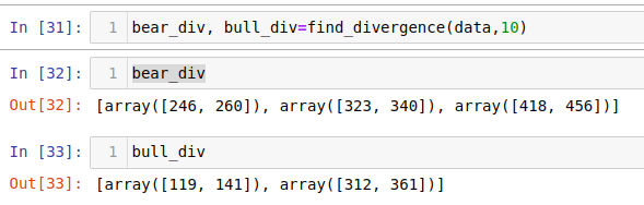
Function returns lists of arrays with coordinates of x-axis for divergence lines. Now it remains for us to plot chart with results.

fig=make_subplots(rows=2, cols=1, subplot_titles=("EUR USD Price", "RSI"))
fig.append_trace(go.Scatter(x=data.index, y=data['c'].values, mode='lines'), row=1,col=1)
fig.append_trace(go.Scatter(x=data.index, y=data['RSI'].values, mode='lines', line_color='grey'), row=2,col=1)
for h_line in bear_div:
    fig.append_trace(go.Scatter(x=data.iloc[h_line].index, y=data['c'].iloc[h_line], mode='lines', line_color='red'), row=1, col=1)
for l_line in bull_div:
    fig.append_trace(go.Scatter(x=data.iloc[l_line].index, y=data['c'].iloc[l_line], mode='lines', line_color='green'), row=1, col=1)
for h_line_rsi in bear_div:
    fig.append_trace(go.Scatter(x=data.iloc[h_line_rsi].index, y=data['RSI'].iloc[h_line_rsi], mode='lines', line_color='red'), row=2, col=1)
for l_line_rsi in bull_div:
    fig.append_trace(go.Scatter(x=data.iloc[l_line_rsi].index, y=data['RSI'].iloc[l_line_rsi], mode='lines', line_color='green'), row=2, col=1)
fig.update_xaxes(rangebreaks=[dict(bounds=['sat', 'mon'])])
fig.show()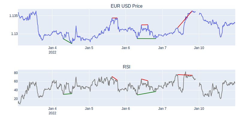

RSI divergence as trading strategy

If we are able to define divergence on price chart and RSI chart, let’s try to define, it as standalone trading strategy.

def rsi_divergence(data, freq, window, order, plot_data={2:[('RSI',None,'blue')]}):
    
    df=data.copy()
    
    freq = f"{freq}min"
    df = df.resample(freq).agg({"Open": "first", "High": "max", "Low": "min", "Close": "last",  'spread':'mean','pips':'mean'}).dropna()
    
    df["returns"] = np.log(df['Close'] / df['Close'].shift(1))
    
    #calculating RSI with talib
    df['RSI']=ta.RSI(df['Close'], window)
    
    bear_div, bull_div=find_divergence(df, order)
    
    bear_points=[df.index[a[1]] for a in bear_div]
    bull_points=[df.index[a[1]] for a in bull_div]
    
    pos=[]
    
    for idx in df.index:
        if idx in bear_points:
            pos.append(-1)
        elif idx in bull_points:
            pos.append(1)
        else:
            pos.append(0)
    
    df['position']=pos
    
    df['position']=df['position'].replace(0, method='ffill')
    
    
    return df

Python code follows the convention from other strategies defined in Strategies.py. So, as arguments should be passed: data, frequency of data, window range for calculate RSI and order to find local highs and lows of price . After that with find_divergence function, reversal points are appointed. When it is done, we will just create position column with reversal points. Now let’s test strategy with StrategyTester.py .

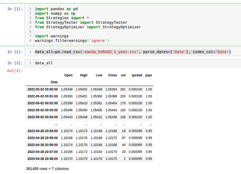
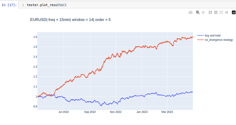
Range of data is one year with frequency of 1 minute. Data is ready to be tested with RSI divergence trading strategy.

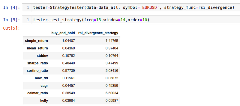
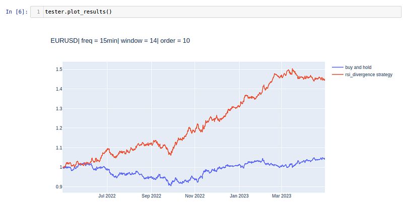
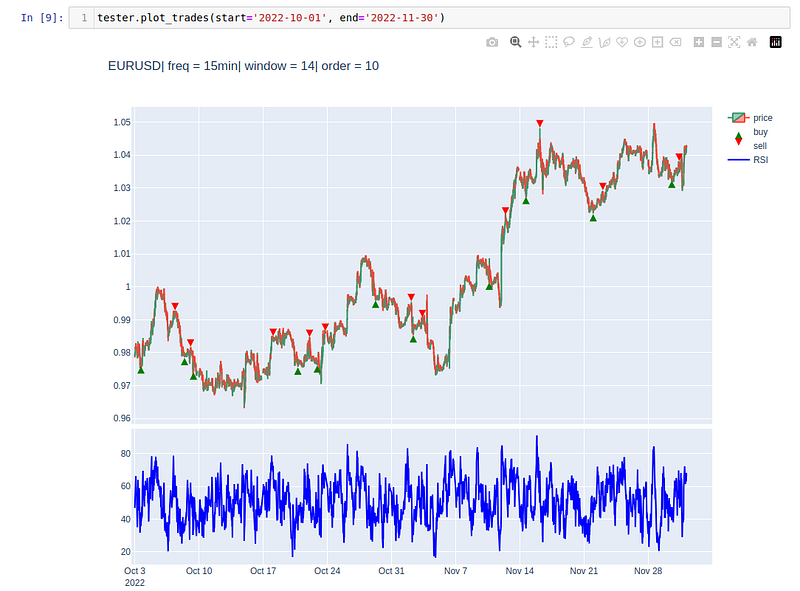
Results of strategy looks quite good with historical data. Let’s see results on the chart.

To see example trades, we can use plot_trades method. For better readability of chart I have limited range of data.

Strategy optimization

Parameters for RSI divergence trading strategy can be optimizing using StrategyOptimizer.py class.

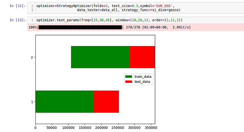
Data that was used to optimize parameters, are marked on the bar chart as green horizontal bars. We have tested 270 combinations of parameters, but of course you can define broader range of parameters to be tested. Now let’s see dataframe with results.

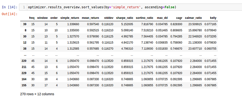
The optimal parameters for this set of data, are, freqency of 15 minutes, window for RSI — 14 and order of 10 for argrelextrema function. And we can test these optimal parameters again on whole dataset.

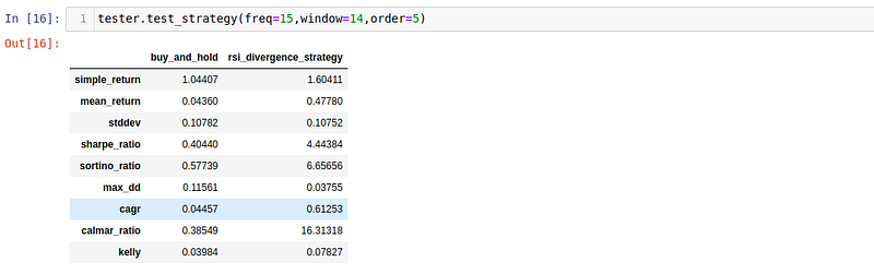
And last point of this article is plot chart with return from strategy with optimal parameters.

Whole explanation of how to optimize trading strategy you can find in this article

As you can see even standalone RSI divergence trading strategy looks promising. But I have to notice again, that it looks like that only for this set of data.

More you can find on my github .

This article is not investment advice. The information contained on this website and the resources available for download through this website are for educational and informational purposes only.

A Message from InsiderFinance

Thanks for being a part of our community! Before you go:

• 👏 Clap for the story and follow the author 👉
• 📰 View more content in the InsiderFinance Wire
• 📚 Take our FREE Masterclass
• 📈 Discover Powerful Trading Tools