Road Map from Naive Bayes Theorem to Naive Bayes Classifier (Stat-09)

Complete Guideline for Naive Bayes Classifier with Implementation from Scratch

The name Naive Bayes itself expresses the meaning of the algorithm. But how! Let’s analyze the name of the algorithm, Naive Bayes. We find two terms, one is Naive, and another is Bayes. Here, Naive means all the features used in algorithms are independent of each other; moreover, it is called Bayes because it depends on Bayes theorem. A naive Bayes classifier is a collection of classifier algorithms where all of them share a common principle as each of the feature pairs are classified independently of each other. It predicts based on an object. To understand the algorithm, we have to begin with some basic terminologies such as Generative Model, Bayes Theorem. There are two types of Machine Learning models.

Generative Model
Discriminative Model

The Naive Bayes classifier is one of the use cases of the generative model. So at the very beginning, we will discuss the generative model.

[N.B. Before reading the article, I suggest you to go through the following article if you want to know about the concepts of probability.]

Basic Probability Concepts for Data Science

Probability Helps to Predict the Unknown Outcome of Any Event

towardsdatascience.com

✪ Generative Model

The generative model mainly focuses on the distribution of the data, and it calculates the class considering the density of the distribution.

Some Examples of Generative Model:

‌Naïve Bayes
Bayesian networks
Markov random fields
‌Hidden Markov Models (HMMs)
Latent Dirichlet Allocation (LDA)
Generative Adversarial Networks (GANs)
Autoregressive Model

✪ Bayes Theorem

Bayes theorem, named after British mathematician Thomas Bayes, was used to find conditional probability. Conditional probability is used to find the event probability based on the previous event. Bayes theorem generates posterior probability to dissection prior probability.

Prior probability is the likeness of an event before taking a new data point.

The posterior probability is the presumption of an event after taking a new data point. Decisively, the Bayes theorem tries to find the likelihood of the event after new data or information is added to the dataset. The formula for Bayes theorem :

P(A|B) = P(A) * P(B|A)/P(B)

Where,

P(A) denotes probability of occurring of an event A

P(B) denotes probability of occurring of an event B

P(A|B) denotes probability of occurring A when B is given

P(B|A) denotes probability of occurring B when A is given

◉ How Naive Bayes Algorithm Work

A classification problem might have one, two, or more class labels. Suppose we have m class labels y1, y2, …, ym, and n input variables X1, X2, …, Xn. From these data, we may calculate the probability of given input variables. The formula for the data would be as follows–

P(yi | x1, x2, …, xm) = P(x1, x2, …, xn | yi) * P(yi) / P(x1, x2, …, xm).

We have to determine the values yi where i =1,2,….,m. At last, Compare these Probability values with corresponding yi values. The maximum probability value denotes the output labels.

Let’s make it easier with the following example. Suppose we have a ‘ weather condition’ dataset consisting of three input variables, Outlook, Temperature and Humidity, and corresponding target value ‘Play’. We are trying to find the probability of playing on a particular day based on input variables. Assume we have to calculate the probability of playing for the weather condition: Outlook=Sunny, Temperature = Cool, Humidity = Normal.

In the beginning, we have to convert the dataset in a frequency table for particular input variables and also calculate the likelihood:

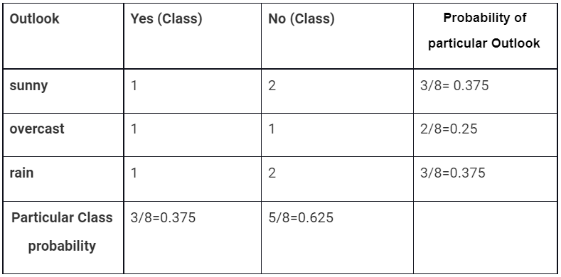
➣ For Outlook input variable

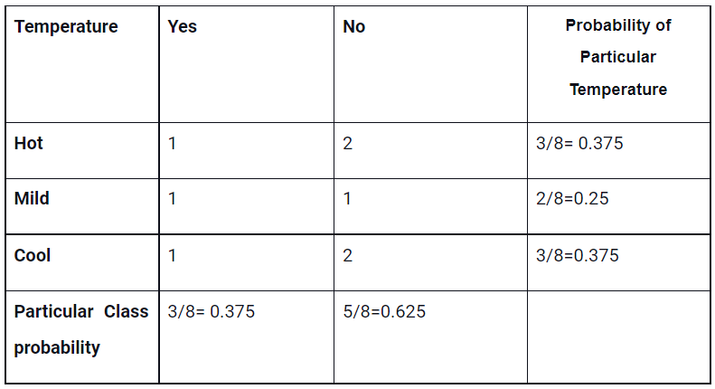
➣ For the Temperature input variable

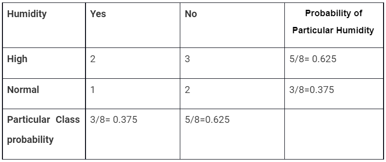
➣ For humidity input variable

Here, P(play = yes) = 0.5 and P(play =no) = 0.5

Now, our recipe is ready to apply Bayes Theorem to find the output of whether on that rainy day players will play or not.

P(Yes|sunny,......high)=P(sunny|Yes)*P(cool|Yes)*P(Normal|Yes)*P(Yes)/(P(sunny)*P(cool)*P(Normal)

From the above tables

P(sunny|Yes)= 1/4 = 0.25

P(cool|Yes)=2/4 = 0.5

P(Normal|Yes)=2/4 = 0.5

P(sunny) = 0.375

P(cool)= 0.375

P(Normal) = 0.375

P(Yes)=4/8 = 0.375

So P(Yes|sunny,…..high) = (0.25*0.5*0.5*0.375)/(0.375*0.375*0.375)= 0.444

P(No|sunny……high)= P(sunny|No)*P(cool|No)*P(Normal|No)*P(No)/(P(sunny)*P(cool)*P(Normal))

From above tables

P(sunny|No)= 1/4 = 0.25

P(cool|No)=2/4 = 0.5

P(Normal|No)=2/4 = 0.5

P(sunny) = 0.375

P(cool)= 0.375

P(Normal) = 0.375

P(No)=4/8 = 0.625

So P(No|sunny,…..high) = (0.25*0.5*0.5*0.625)/(0.375*0.375*0.375)= 0.740740

So, we have found from the above calculation.

P(No|sunny,…..high) > P(No|sunny,…..high)

Hence, on a Rainy day, the Player can’t play the game.

✪ Types Of Naive Bayes Model

Types of naive Bayes models are based on their distribution. Such as

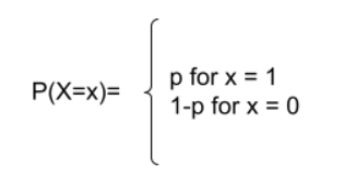
◉ Bernoulli Naive Bayes

Bernoulli Naive Bayes is an important naive bayes algorithm. This model is famous for document classification tasks where it determines if a particular word stays in the document or not. In these cases, the counting of the frequency is less important. It is the most simplified algorithm. This algorithm is most effective for small datasets. The decision rule for Bernoulli naive Bayes is

For example, you want to know whether a document contains a particular word or not. In this type of binary classification such as True or False, Success or Fail, 0 or 1, Play or Not playing, etc., use Bernoulli Naive Bayes Classification.

◉ Multinomial Naive Bayes

When we investigate the buzz word ‘Multinomial,’ its meaning is closely related to multiclass classification. Suppose you are interested in the frequency of a particular output; Multinomial Naive Bayes is a suitable algorithm for this problem. Another example is that you have given a text document to find the number of occurrences of a particular word in the document. In that situation, you have to apply the multinomial naive Bayes algorithm. For the Multinomial Naive Bayes Algorithm, the Multinomial Distribution Function is used. The multinomial distribution Function:

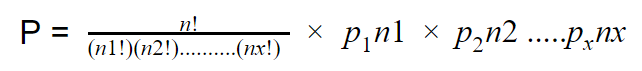
Here, we will show the equation and find the process of P using a solid example below. For instance, We have collected a sample of blood groups from the city’s population (Rajbari, Dhaka, Bangladesh). Also, calculate the probability for each blood group in the sample.

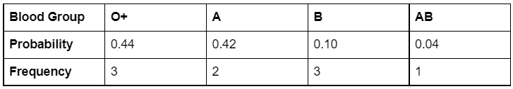
Now, you have given a problem, take 9 people randomly and calculate.

Here, n1= the frequency value of O+,

n2 = the frequency value A,

n3 = the frequency value B ,

n4 = the frequency value AB

Here, n=9, the total number of random samples.

Also,p1 = 0.44 = the probability blood group O+ in the sample,

p2=0.42=the probability of blood group A in the sample,

p3=0.10=the probability of blood group B in the sample,

p3=0.04=the probability of blood group AB in the sample

Now, Just put the above values into the equation, and you will get the probability of multinomial Naive Bayes.

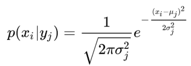
◉ Gaussian Naïve Bayes

Bernoulli Naive Bayes and Multinomial Naive Bayes are used for discrete type datasets. But we will work with a real-world dataset that is continuous data. In this case, we need to use the Gaussian Naive Bayes theorem. The Gaussian Distribution or Normal Distribution function seems as follows:

✪ Implementation Of Naive Bayes Algorithm From Scratch

In order to implement Naive Bayes from scratch, we will approach step by step :

#importing necessary libraries
import numpy as np 
import pandas as pd

➣ Creating a dataset for implementing Naive Bayes algorithm from scratch.

from sklearn.datasets import load_breast_cancer
cancer = load_breast_cancer()

data = pd.DataFrame(data=cancer.data, columns=cancer.feature_names)
data['diagnosis'] = cancer.target

data = data[["mean radius", "mean texture", "mean smoothness", "diagnosis"]]
data.head(10)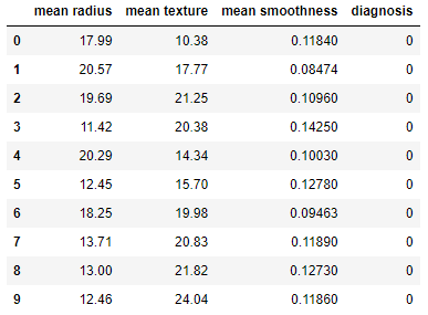

➣ Firstly, we have to calculate the prior probability. We have created a function calculate_prior_probability where you take data frame, df, and Y as an input and return prior probability value. Such as P(Y=Yes) or P(Y=No).

➣ We have to calculate the conditional probability as we create the function cal_likelihood_gau. We will input the necessary data to calculate the probability of input variable X when Y labels are given, which means probability X is given Y. The function returns pro_x_given_y, which will be used further.

➣ Finally, You have to build the model and calculate posterior probability using the previous two functions calculate_prior_probability and cal_likelihood_gau.

➣ Predicting the final output form the above naive_bayes_gaussian() function.

Output

[[36  4]  
 [ 0 74]] 
0.9736842105263158

✪Implementation of Naive Bayes Algorithm Using Sckit-learn

➣ Importing the necessary libraries for implementing the Naive Bayes algorithm using Sckit-learn. Here, we will implement Bernoulli, Gaussian, and Multinominal Naive Bayes algorithm.

from sklearn import metrics
import urllib
from sklearn.naive_bayes import BernoulliNB,GaussianNB, MultinomialNB
from sklearn.metrics import accuracy_score
from sklearn.model_selection import train_test_split

➣ Splitting the dataset for train, test and transforming the data to the fit the model.

train, test = train_test_split(data, test_size=.2, random_state=41)
X_train=train.iloc[:,:-1].values
y_train=train.iloc[:,-1].values
X_test = test.iloc[:,:-1].values
y_test = test.iloc[:,-1].values

➣ Finally, train the models,testing the accuracy and showing the confusion metrics.

Output

0.6491228070175439 
0.7368421052631579 
0.9649122807017544 
0.9736842105263158 
[[36  4]  
 [ 0 74]]

The above result clearly indicates that the Gaussian Naive Bayes algorithm outperforms comparing other Naive Bayes algorithms as the dataset contains the continuous value.

Source: https://upload.wikimedia.org/wikipedia/commons/b/b4/Naive_Bayes_Classifier.gif

The above gif demonstrates how the Naive Bayes Classifier works.

Conclusion

Naive Bayes classifier is an easy, simple but powerful classification algorithm in supervised learning. It performs well where the classification provides effective results if we consider the distribution of the dataset. More precisely, when there is the dependency on the previous occurrences of an event. In natural language processing, sometimes the algorithm shows a promising result.

References

1.https://www.analyticsvidhya.com/blog/2017/09/naive-bayes-explained/

2.https://www.javatpoint.com/machine-learning-naive-bayes-classifier