RNNs, LSTMs, CNNs, Transformers and BERT

Recurrent Neural Networks (RNNs)

RNNs do have memory to keep track of things, so they allow information to be persistent over the network. Look at the given below picture. The left side of the image shows one RNN cell which accepts some input say x and process within a hidden cell h and finally responds with an output o. Apart from being linear, a loop within the hidden layer allows data to be sent to the next layer. Collectively, we could say like RNN is a group of similar network chunks. If we unfold the left image, we would get something like given in the right side. We give data to each input cell and output of the previous cell. For instance, to the second network chunk we input Xt and Ot-1 which is the output of previous chunk.

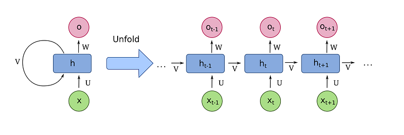
The chain like structure shows that recurrent neural networks are clearly related to sequences. In that way, if we want to convert some text from one language to another, we can set each word as the input. The RNN passes the information of previous cell to the next cell which could be used to understand the context of the sentence.

Let’s think about a scenario, suppose we’re building a language model which predicts the next word in a sentence based on the previous ones. If we are taking care of the sentence “machine learning is the subset of AI’, we don’t need to worry much about the context i.e. “AI” is coming after the word “of”. In this case, the place where the context is required and the relevant information is negligibly narrow. But this scenario changes drastically when we encounter something like “I was born and brought up in US. I have a bachelor’s from Standford…, I speak fluent …..”, we really know that, the next word would be English- most probably because we have that information like he was born and brought up in US where English is the native language. This assumption might really help us in making the prediction. As compared to the previous example, the difference between the place where the prediction is expected and the relevant information is too high. We need to keep the context active from the first ever sentence to the last. RNNs are too sensitive to the overall length of the data, i.e. it hardly performs in such cases where the above mentioned gap is high. RNNs won’t scale much where long term dependencies are required. This is due to the fact that, information is lost when the chain becomes too long and it fails to keep track of the overall context.

Long - Short Term Memory (LSTMs)

When some new information is added to the RNN, it transforms the existing information to a whole new version of it by applying some formulations. So there won’t be a consideration among what is important and what is not much. Long - Short Term Memory (LSTM) always keep track of this issue by using a mechanism called cell state. So the LSTMs can remember like oh .. this information is required and this is not that much. LSTMs have a similar structure as given below.

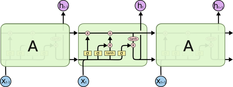
Each cell of Xt-1, X and Xt+1 take different inputs and does some operations on it. Rather than the original input alone, each cell conceives the state and output of the previous cell, then it generates a new cell state and output which would eventually transmitted to the very next cell and so goes on.

The same problem of RNNs still exists here, i.e. as the input becomes broader or the length increases, LSTMs also fail to keep the relevant information active. Keeping the context of a word which is faraway from the place where it is required becomes too difficult because the cell must have forgotten or the cell state must have rewritten. The importance of words would decrease as it move along.

Another problem with both RNNs and LSTMs is, they can’t do the task in parallel. That is, in the case of a language translation model, each word is sent to the network sequentially. The time takes to calculate something would really be depended on the overall length of the text since each word is given as the input to the network.

Convolutional Neural Networks (CNNs)

Convolutional Neural Networks (CNNs) can help us with parallelization, local dependencies and distance between positions.

Some of the widely used neural networks for sequence transduction such as Wavenet and Bytenet are CNNs.

The reason why CNNs can work in parallel is that, each word on the input can be processed at the same time and does not necessarily depend on the previous words to be translated. Not only that, but the “distance” between the output word and any input for a CNN is in the order of log(N) —i.e. size of the height of the tree generated from the output to the input (you can see it on the GIF above). That is much better than the distance of the output of a RNN and an input, which is in the order of N.

Transformers

Transformers were introduced to deal with the long-range dependency challenge. It was proposed in this paper.

From the paper,

The Transformer is the first transduction model relying entirely on self-attention to compute representations of its input and output without using sequence-aligned RNNs or convolution.

Here, transduction means the conversion of input sequences into another format, in our example it is the translation of a sentence from one language to another. Let’s see how a transformer looks like.

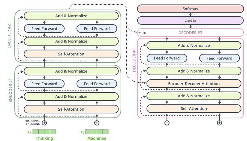
The major components of a transformer are a set of encoders and decoders. Encoders encode input into a representation which then decoded by the decoders. One encoder block has a self-attention mechanism and a feed forward neural network. On the other hand, a decoder has both the components of an encoder and an encoder - decoder attention, in addition. The encoders and decoders are stacks of identical structures, i.e there will be a couple of encoders stacked one on the top of another. In the same way, a number of decoders would also be stacked together. The word embeddings of the input sequence would be passed to the first encoder. These are then transformed and sent to the very next encoder and so on. The output of the final encoder would be the input of first decoder, this decoder then applies some transformations and would be sent to the next decoder.

Here the question is, what is really meant by self-attention. According to the original paper,

Self-attention, sometimes called intra-attention, is an attention mechanism relating different positions of a single sequence in order to compute a representation of the sequence.

Self-attention allows models to look at other words in the input sequence to get a better understanding of a certain word in the sequence.

Here you can find the visual explanation of transformers and the different calculations carried out to find the self-attention score.

Bidirectional Encoder Representations from Transformers (BERT)

BERT is backed by Transformer and it’s core principle - attention, which understands the contextual relationship between different words. Rather than decoding the encoded information, BERT only encodes and generates a language model, so an encoder is enough. As compared to directional models such as RNN and LSTM which conceive each input sequentially (left to right or right to left). In fact, Transformer and BERT are non-directional - to be very precise, because both these models read the whole sentence as the input instead of sequential ordering. This characteristic allows models to learn the contextual information of a word with respect to all other words in the sentence.

Bert uses two training mechanisms namely Masked Language Modeling (MLM) and Next Sentence Prediction (NSP) to overcome the dependency challenge.

Masked Language Modeling (MLM)

Before feeding the input vector into the encoder, 15% of the words in the sequence will be masked with a [MASK] token. For instance, the sentence “I love my kitty” would be represented as “I love my [MASK]” and note that all words will be replaced with it’s vector representation. The goal of MLM is to predict the masked word with respect to all other words in the sentence.

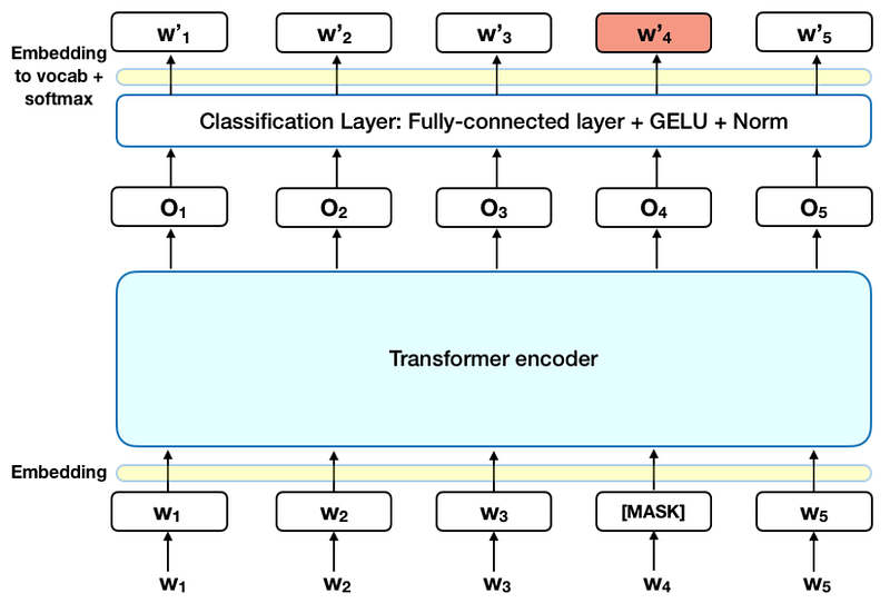
From the figure, we can observe like encoded output of the Transformer encoder is sent to a fully connected classification layer. The results of the classifier would then be multiplied by an embedding matrix to convert to the vocabulary and finally a softmax scoring is done to see the predicted probability of the words. The loss or cost function only takes care of the predictions of the masked terms. So it would take too much time to converge into it’s optimum.

Next Sentence Prediction (NSP)

While training, the model would receive pairs of sentences as inputs. Out of the whole input pairs, 50% of them would have the exact consecutive sentence as the second term and the rest of them would have random sentences as the second sentence. The model eventually learns it and predicts whether the second sentence in the pair is actually the consecutive sentence or not. The assumption is, the sentence which was chosen randomly would be disconnected from the first. Each input undergoes some pre-processing precedure before being fed into the model. Look at the figure below.

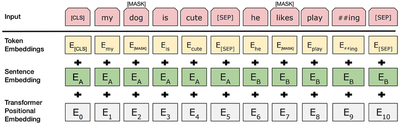
We can understand, a[CLS] token at the beginning and a [SEP] token at the end of a sentence are added. Token embeddings are then added with sentence embeddings - indicating the current sentence A or B. Finally a positional embedding is added to each token to indicate it’s position in the sentence. To predict whether the second sentence is connected to the first sentence, the entire input sequence would be sent to a Transformer encoder and then the output of the [CLS] token is transformed into a 2×1 shaped vector, using a simple classification layer (learned matrices of weights and biases). A softmax function is added at the end to see the probability of the prediction.

When training the BERT model, Masked LM and Next Sentence Prediction are trained together, with the goal of minimizing the combined loss function of the two strategies.

Thanks for the time!