RL — Value Learning

Value learning is a fundamental concept in reinforcement learning RL. It is the entry point to learn RL and as basic as the fully connected network in Deep Learning. It estimates how good to reach certain states or to take certain actions. While it may not be sufficient to use value-learning alone to solve complex problems, it is a key building block for many RL methods. In this article, we will use examples to demonstrate its concept.

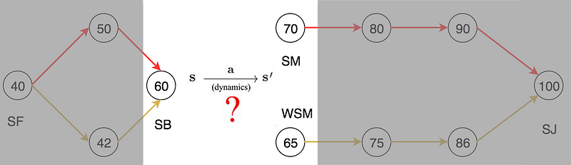
Let’s plan a trip from San Francisco to San Jose. Say you are a devoted data scientist and you include many factors in your decision. These factors may include the remaining distance, the traffic, the road condition and even the chance of getting a ticket. After the analysis, you score every city and you always pick the next route with the highest score.

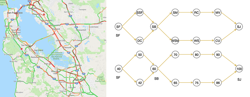
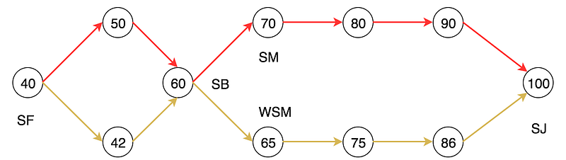
For example, when you are in San Bruno (SB), you have two possible routes. Based on their scores, SM has a higher score and therefore, we will travel to SM instead of WSM.

In reinforcement learning RL, the value-learning methods are based on a similar principle. We estimate how good to be in a state. We take actions for the next state that will collect the highest total rewards.

Value function

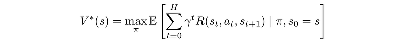
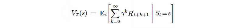
Intuitively, value function V(s) measures how good to be in a specific state. By definition, it is the expected discounted rewards that collect totally following the specific policy:

where γ is the discount factor. If γ is smaller than one, we value future rewards with a lower current value. In most of the examples here, we set γ to one for simplicity in illustration. Our objective is finding a policy that maximizes the expected rewards.

There are many methods to find the optimal policy through value learning. We will discuss them in the next few sections.

Value iteration

First, we can use dynamic programming to calculate the optimal value of V iteratively.

Then, we can use the value function to derive the optimal policy.

When we are in SB, we have two choices.

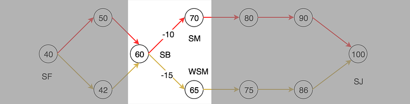
The SB to SM route receives a -10 rewards because SB is further away. We get an additional -5 rewards for the SB to WSM route because we can get a speeding ticket easily in that stretch of the highway.

The optimal V*(SB) = max( -10 + V*(SM), -15 + V*(WSM)) = 60.

Value Iteration Example

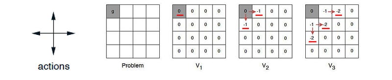
Let’s get into a full example. Below is a maze with the exit on the top left. At every location, there are four possible actions: up, down, left or right. If we hit the boundary, we bounce back to the original position. Every single-step move receives a negative one reward. Starting from the terminal state, we propagate the value of V* outwards using:

The following is the graphical illustration from iteration one to seven.

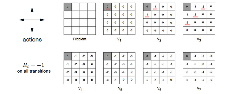
Once it is done, for every location, we locate the neighbor with the highest V-value as our best move.

Policy evaluation

The second method is the policy evaluation. A policy tells us what to do from a particular state.

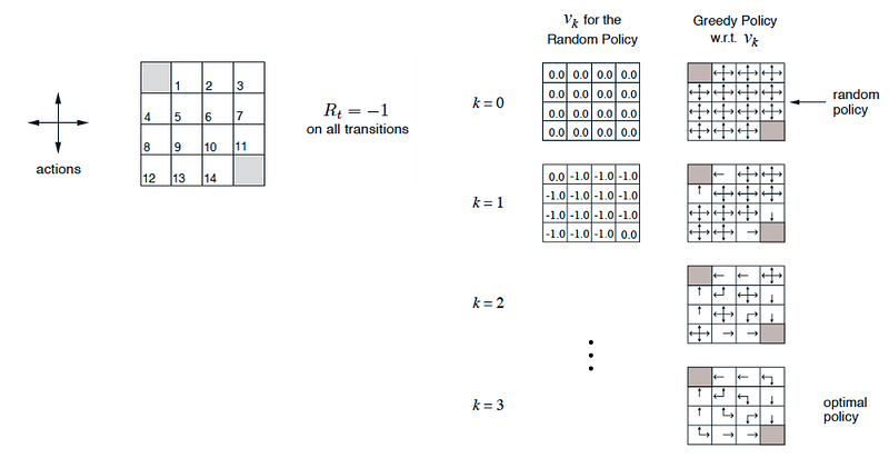
We can evaluate a random policy continually to calculate its value functions. A random policy is simply a policy that take any possible action randomly. Let’s consider another maze with exits on the top left and the bottom right. The value function is calculated as:

For a random policy, each action has the same probability. For four possible actions, π(a|s) equals 0.25 for any state.

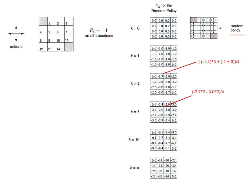
For iteration 3 below, V[2, 2] = -2.9: we subtract one from each neighbor (negative one reward for every move), and take their average.

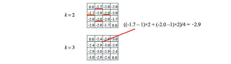
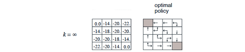
As we continue the iteration, V will converge and we can use the value function to determine the optimal policy again.

Policy Iteration

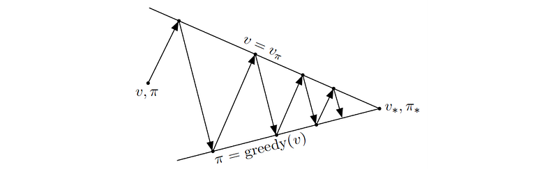
The third method is the policy iteration. Policy iteration performs policy evaluation and policy improvement alternatively:

We continuously evaluate the current policy but we also refine the policy in each step.

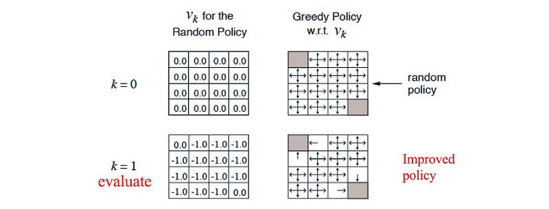
As we keep improving the policy, it will converge to the optimal policy.

Here is the example which we can find the optimal policy in four iterations, much faster than the policy evaluation.

Algorithm

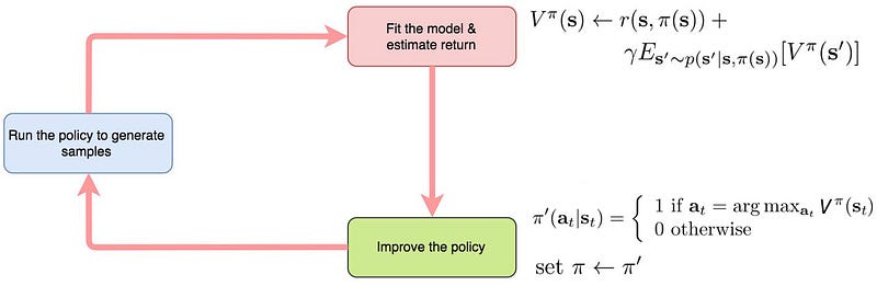
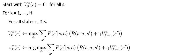
Let’s formulate the equations. The value-function at time step i+1 equals

Where P is the model (system dynamics) determining the next state after taking an action. The refined policy will be

For a deterministic model, the equation can be simplified to:

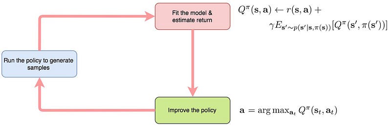
Here is the general flow of the algorithm:

Bellman Optimality Equation

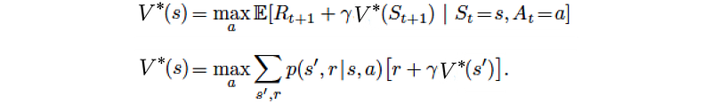
In the previous section, we use the dynamic programming to learn the value iteratively. The equation below is often mentioned in RL and is called the Bellman equation constraint.

Value-Function Learning with Stochastic Model

In the previous value iteration example, we spread out the optimal value V* calculation to its neighbors in each iteration

using the equation:

In those examples, the model P is deterministic and is known. P is all zero except one state (s’) that is one. Therefore, it is simplified to:

But for the stochastic model, we need to consider all possible future states.

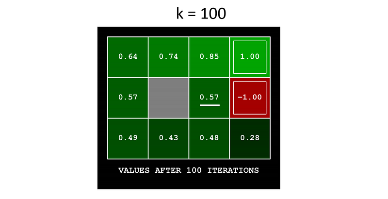
Let’s demonstrate it with another maze example using a stochastic model. This model has a noise of 0.2. i.e., if we try to move right, there is 0.8 chance that we do move right. But there is a 0.1 chance that we move up and 0.1 chance that we move down instead. If we hit a wall or boundary, we bounce back to the original position.

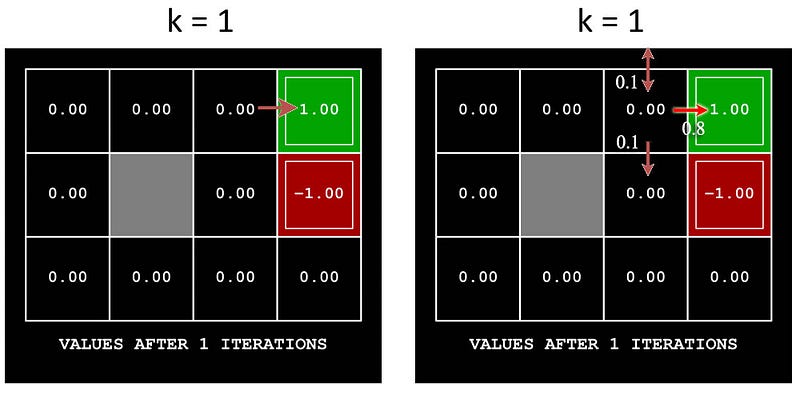
We assume the discount factor γ will be 0.9 and we receive a zero reward for every move unless we hit the terminate state which is +1 for the green spot and -1 for the red spot above.

Let’s fast forward to iteration 5, and see how to compute V*[2, 3] (underlined in white below) from the result of iteration 4.

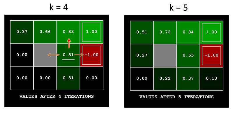
The state above [2, 3] has the highest V value. So the optimal action for V*[2, 3] is going up. The new value function is

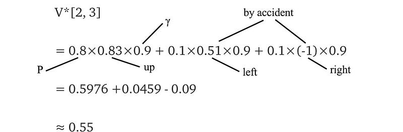
In each iteration, we will re-calculate V* for every location except the terminal state. As we keep iterating, V* will converge. For example, V*[2, 3] eventually converges to 0.57.

Algorithm

Here is the pseudocode for the value iteration:

Model-Free

Regardless whether it is a deterministic or a stochastic model, we need the model P to compute the value function or to derive the optimal policy. (even though in a deterministic model, P is all zero except one state which is one.)

Monte-Carlo method

Whenever we don’t know the model, we fall back to sampling and observation to estimate the total rewards. Starting from the initial state, we run a policy and observe the total rewards (G) collected.

G is equal to

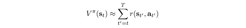
If the policy or the model is stochastic, the sampled total rewards can be different in each run. We can run and reset the system multiple times to find the average of V(S). Or we can simply keep a running average like the one below so we don’t need to keep all the previous sampled results.

Monte-Carlo method samples actions until the end of an episode to approximate total rewards.

Monte-Carlo control

Even we can estimate V(S) by sampling, how can we determine the action from one state to another?

Without knowing the model, we don’t know what action can lead us to the next optimal state s’. For example, without the road signs (the model), we don’t know whether the left lanes or the right lanes of the highway lead us to SM or WSM?

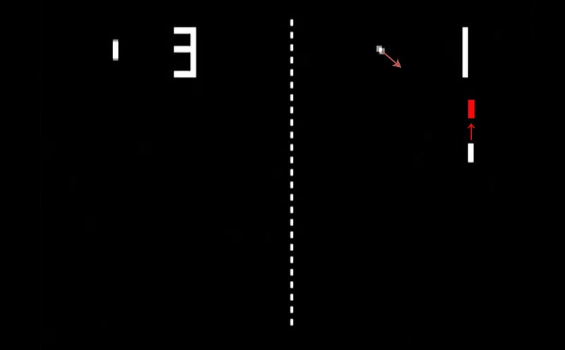
In the pong game below, we know what state we want to reach. But without the model, we don’t know how far (or how hard) should we push the joystick.

Action-value Learning

This comes to the action-value function, the cousin of value function but without the need of a model. Instead of measuring how good a state V(s) is, we measure how good to take an action at a state Q(s, a). For example, when we are at SB, we ask how good to take the right lanes or the left lanes on Highway 101 even though we don’t know where it leads us to. So at any state, we can just take the action with the highest Q-value. This allows us to work without a model at the cost of more bookkeeping for each state. For a state with k possible actions, we have now k Q-values.

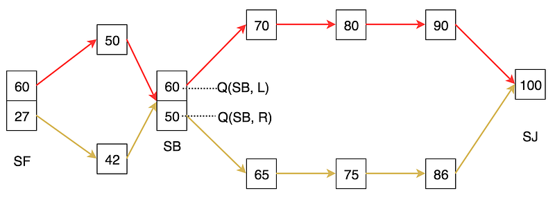
The Q-value (action-value function) is defined as the expected rewards for an action under a policy.

Similarly to the previous discussion, we can use the Monte-Carlo method to find Q.

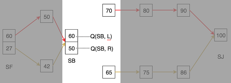
In our example, we will keep on the left lanes when we are in SB.

This is the Monte-Carlo method for Q-value function.

Policy Iteration with Q-value (model-free)

We can apply the Q-value function in the policy iteration. Here is the flow:

Issues

The solution presented here has some practical problems. First, it cannot scale well for a large state space. The memory to keep track of V or Q for each state is impractical. Can we build a function estimator for value functions to save memory, just like the deep network for a classifier? Second, the Monte-Carlo method has very high variance. A stochastic policy may compute very different reward results in different runs. This high variance hurts the training. How can train the model with better convergence?

Recap

Before looking into the solution. Let’s recap what we learn. We want to find an optimal policy that can maximize the expected discounted rewards.

We can solve it by computing the value function or the Q-value function:

And this can be solved using dynamic programming:

or one-step lookahead which is also called Temporal Difference TD.

Thoughts

Stay tuned for the next part where we will solve some of the problems mentioned before and apply them in practice.