

RL — Reinforcement Learning Algorithms Quick Overview
This article overviews the major algorithms in reinforcement learning. Each algorithm will be explained briefly in a single context for an easy and quick overview.
Terms
Action-value functions Q, state-value function V and advantage function A are defined as:

Policy Evaluation
Policy evaluation computes the value functions for a policy π using the Bellman equations.
For example,


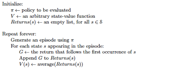
Policy evaluation using Monte Carlo Rollouts
Monte Carlo plays out the whole episode until the end to calculate the total rewards.
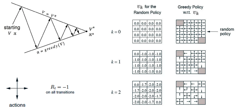
Policy Iteration
Policy iteration evaluates (step 1)

and improves policy (step 2) continuously.


Example: The following maze exits on the top-left or the bottom-right corner with a reward of -1 for every step taken. We evaluate and improve the policy continuously. Since there are only finite actions, the policy will eventually converge to the optimal policy π*.
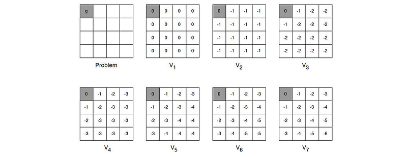
Value Iteration
Compute the value functions iteratively under the Bellman equation using dynamic programming:

Example: This maze exits on the top-left corner with a reward of -1 for every step taken.
Algorithms:

This method ignores the policy and focuses on the value function until the end. The final policy is derived from the value function as:

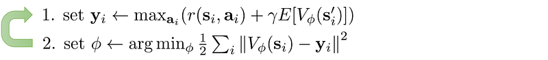
Fitted value iteration
Estimate the value function V with a model parameterized by Φ:
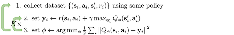
Fitted Q iteration
The Bellman equation for the action-value function is:

Estimate the action-value function Q with a model parameterized by Φ.
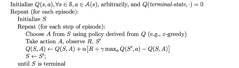
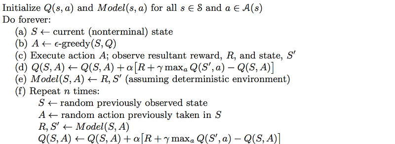
Q-learning (SARSA max)

Q-learning is an online action-value function learning with an exploration policy (like epsilon-greedy).

Pseudocode:
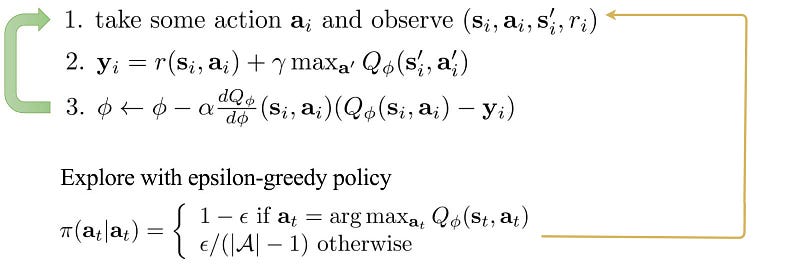
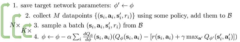
Q-learning with replay buffer and the target network
Add a replay buffer and a target network for training stability.
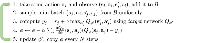
DQN (Deep Q-learning)
DQN is a Q-learning method with a deep network to estimate Q using a replay buffer and a target network.
Policy Gradients
Maximize the rewards by taking actions with high rewards more likely.
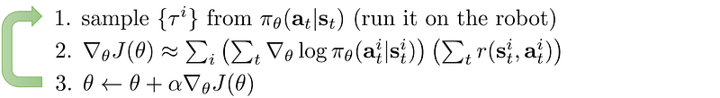
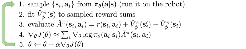
Example: Policy Gradient using Monte Carlo rollouts and a baseline:
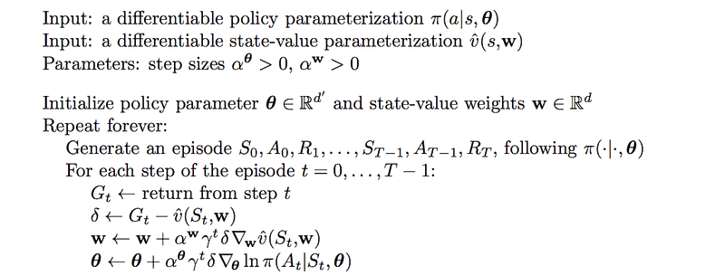
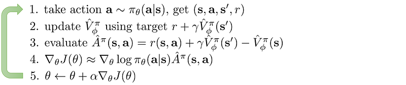
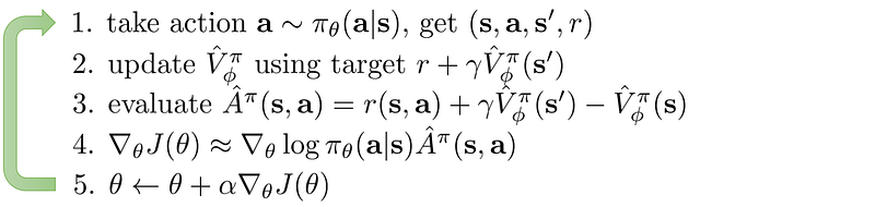
Actor-Critic Algorithm
Combining policy gradient and value-function learning.
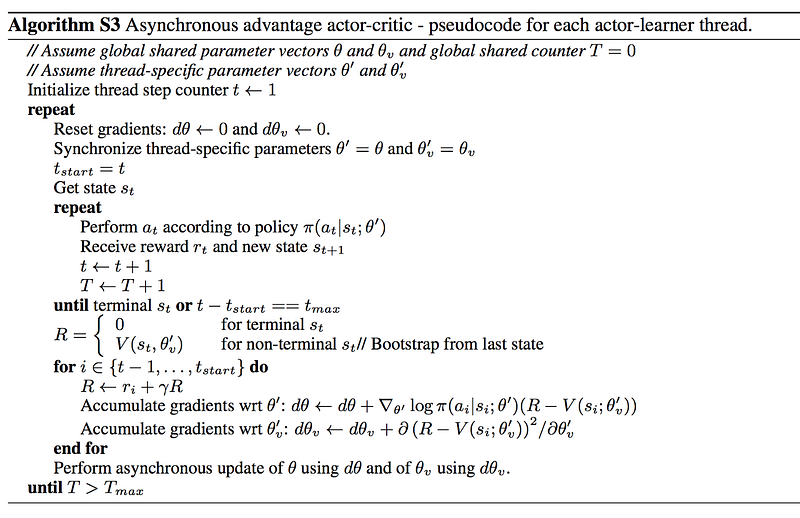
A3C algorithm: asynchronous actor-critic using advantage function.
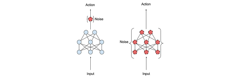
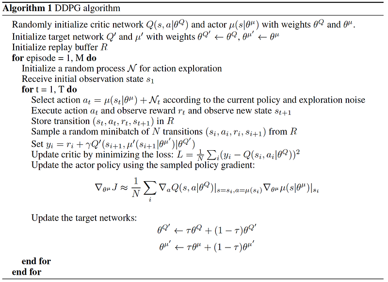
Deep Deterministic Policy Gradient DDPG (Continuous actions)
An actor-critic approach for continuous actions.
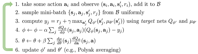
Adding parameter noise for exploration:
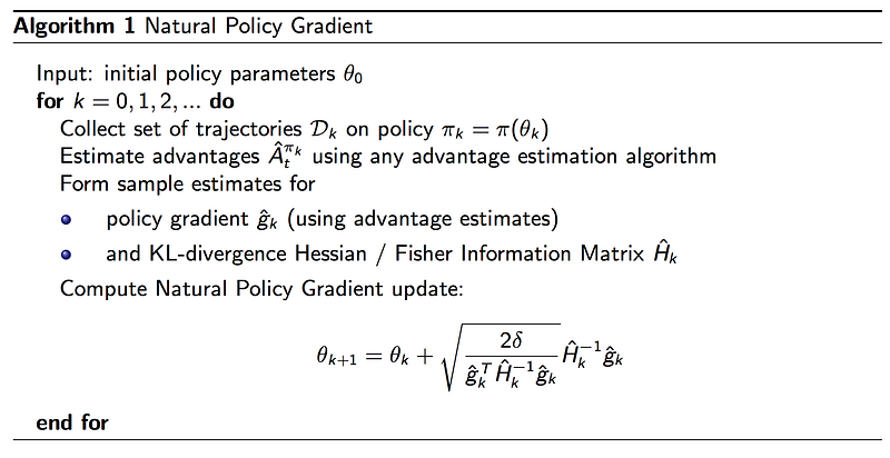
Natural Policy Gradient
Natural Policy Gradient is a better policy gradient method which guarantees policy improvement. It is invariant of how models are created and parameterized.
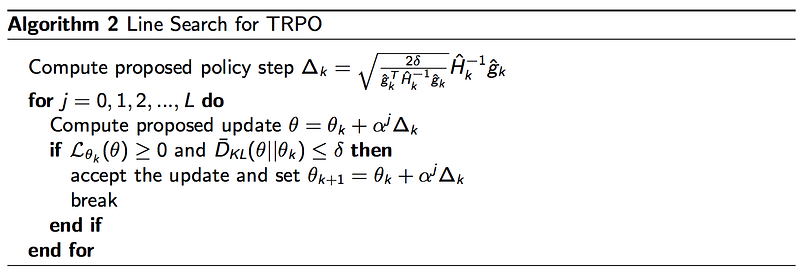
TRPO
Optimize Natural Policy Gradient with Conjugate Gradient.
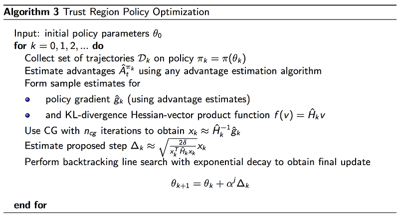
Backtracking line search:
PPO
Optimize Natural Policy Gradient by clipping the advantage function.

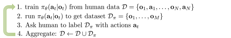
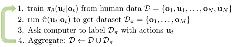
DAgger: Dataset Aggregation
Use human labels to improve imitation learning.
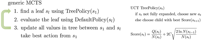
Monte Carlo Tree Search (MCTS)
Search discrete action spaces using a search tree with an exploration tree policy.
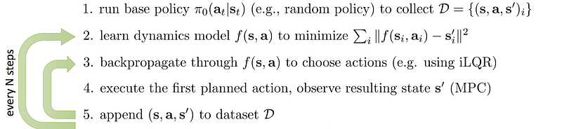
Model-based Reinforcement Learning
MPC (Model Predictive Control)
Replan actions in every action taken.
Policy search with backpropagation
Use backpropagation to build a policy under a model-based method.
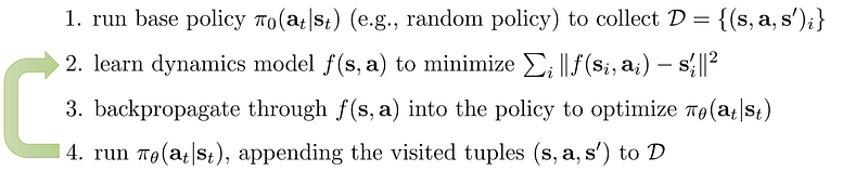
PILCO
Policy search with backpropagation:
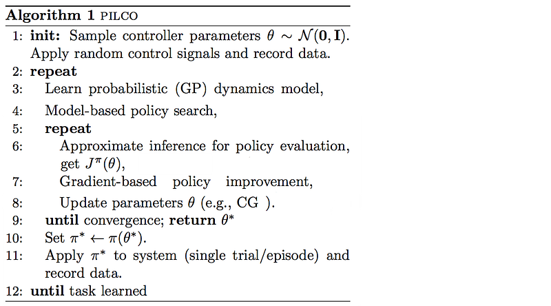
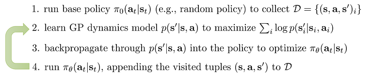
Policy search with Gaussian Process (GP)
Using a Gaussian Process for the dynamic model.
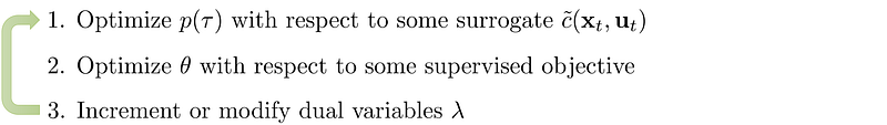
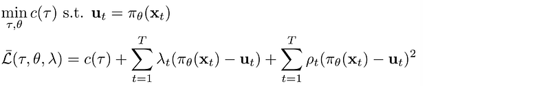
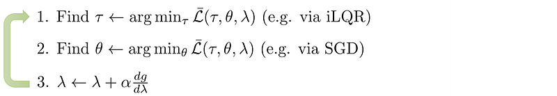
Guided Policy Search (GPS)
General scheme
Use locally optimized trajectory to guide the training of a policy.
Deterministic GPS
Guided Policy Search on deterministic policy.
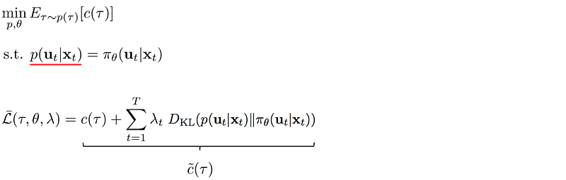
Stochastic GPS
Guided Policy Search on stochastic policy.
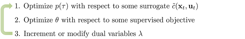
Imitating optimal control
Use computer generated samples (s, a) from locally optimized trajectories to train a policy.
PLATO algorithm
With a Linear Gaussian controller:

We replan with:

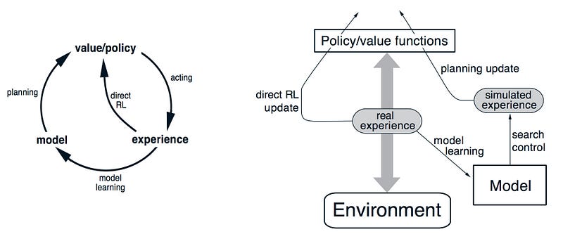
Dyna-Q
Dyna-Q is a constant loop of learning the value function or policy from real and simulated experience. We use the real experience to build and refine the dynamic model, and use this model to produce simulated experience to complement the training of the value function and/or the policy.
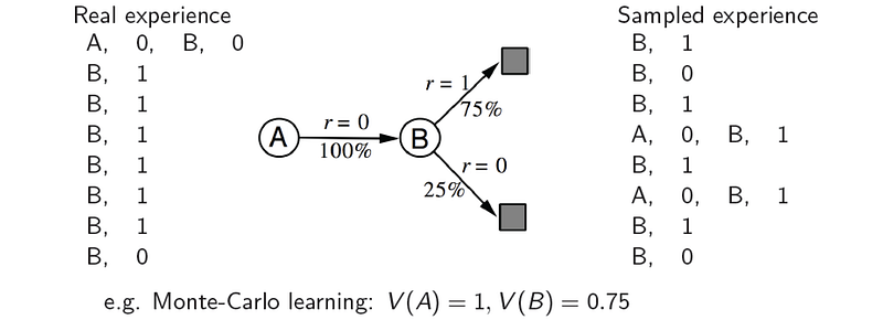
Learned from sampled experience:
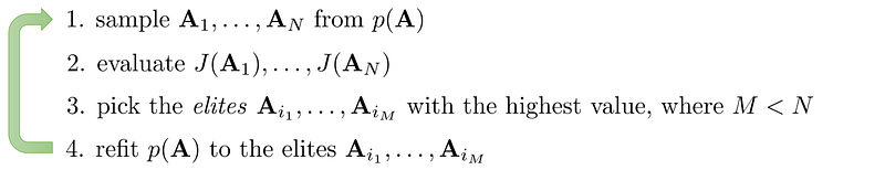
Cross-entropy method (CEM)
Take “educated” random guesses on actions. Select top performers of guesses and use them as seeds for next round of guessing.
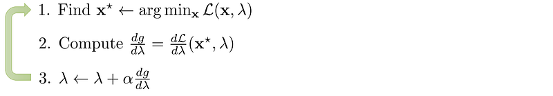
Double Gradient Descent (DGD)
Optimize an objective under constraints.
ε-greedy policy
To sample the kth episode, we use a ε-greedy algorithm below to pick which action to sample next. Here is the data distribution used in selecting the action:

Generalized advantage estimation (GAE)
An n-step look ahead advantage function is defined as:

Advantage function with 1 to k-step lookahead.
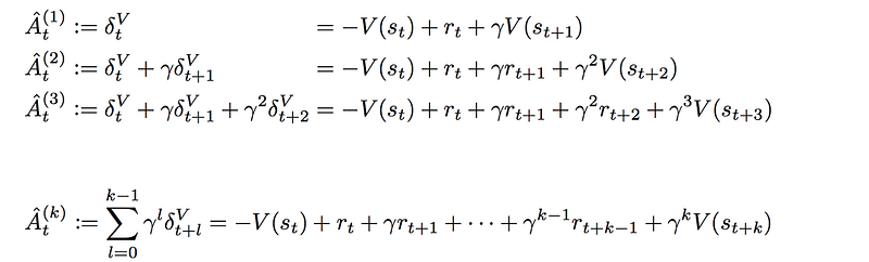
The final advantage function for GAE is

where λ is a hyperparameter from 0 to 1. When λ is 1, it is Monte Carlo. When λ is 0, it is TD with one step look ahead.
Credits and references
UC Berkeley Reinforcement Learning