RL — Optimization Algorithms

This article contains the optimization algorithms often mentioned in RL.

Trust region method

There are two major optimization methods: line search and trust region. Gradient descent is a line search. We determine the descending direction first and we take a step in that direction. In gradient descent, the step size is the gradient × learning rate.

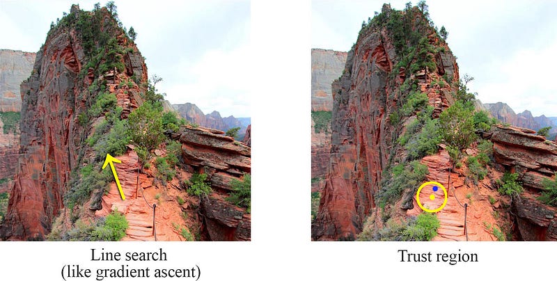
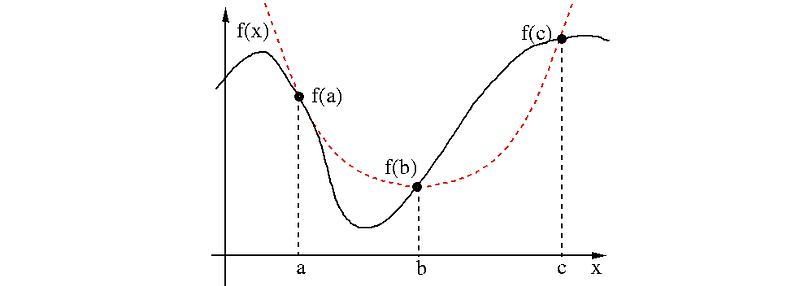
In the trust region, we determine the maximum step size that we want to explore and then we locate the optimal point within this trust region. Let’s start with an initial maximum step size δ as the radius of the trust region (the yellow circle). Our objective is to find the optimal point for m within the radius δ.

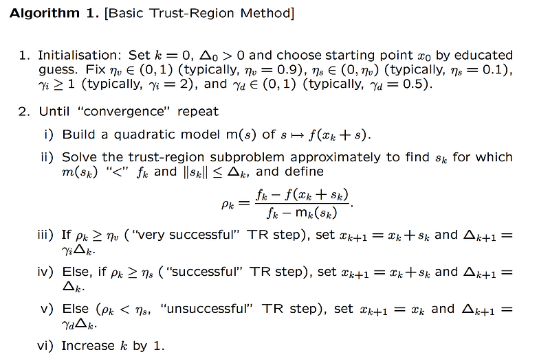
The trust region can be expanded or shrink in runtime to adjust to the curvature of the surface and there are many possibilities. In the traditional trust region method, since we approximate the objective function f with m, one possibility is to shrink the trust region if m is a poor approximator of f at the optimal point. On the contrary, if the approximation is good, we expand it. The following is the trust region method which dynamically adjusts the trust region size according to the criteria just mentioned.

Newton’s method

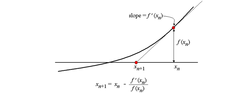
To solve f(x)=0, we can continue the follow iteration until it converges.

It can be used to minimize f(x):

The iteration used will be:

Nonlinear least-squares problem with Gauss-Newton method

(Example credit for the Gauss-Newton method)

Suppose we have a function g(t) model by parameters x1 and x2.

And we have training samples for t with output label y.

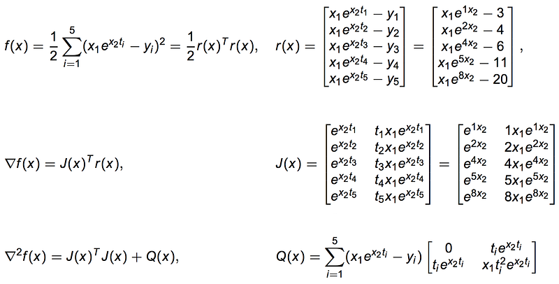
We can define a function r which measures the error between our model and the label:

Now, our objective is to fit our model g with samples to minimize the following objective:

In this section, we will apply the Nonlinear least-squares problem with Gauss-Newton method.

With Newton’s method on optimization:

According to the equation above, we can rewrite the Δx as the searching direction p. The equations becomes:

Compute the first and second order derivative of f:

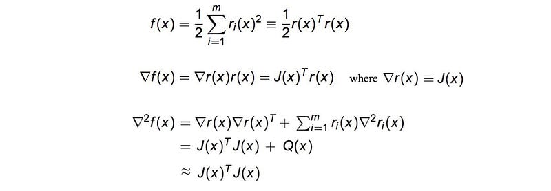
In the Gauss-Newton method, we approximate the second derivative above without the Q term. The Q term is smaller than the first term and if the problem has zero residual, r = Q = 0.

Gauss-Newton method applies this approximation to the Newton method.

The Gauss-Newton method search direction is:

Let’s have an example, we want to determine the growth rate of antelope. We develop a model g and fit data into the model to compute the residual error r: