Ridge, LASSO, and ElasticNet Regression

The continuing adventures of regularization and the eternal quest to prevent model overfitting!

This article is a continuation of last week’s intro to regularization with linear regression. Lettuce yonder back into the nitty-gritty of making the best data science/ machine learning models possible with more advanced techniques on simplifying our models. How do we simplify our models? By removing as many features as possible. Why do I want to do this? I want to have a simpler model. Why do I want a simpler model? Well, because a simpler model generalizes better. What does generalization mean? It means that you can actually use it in the real world. The model does not just explain the training data but it also has a better chance of explaining data that we have not seen before.

Regularization

Regularization seeks to control variance by adding a tuning parameter, lambda, or alpha:

LASSO (L1 regularization)

• regularization term penalizes absolute value of the coefficients
• sets irrelevant values to 0
• might remove too many features in your model

Ridge regression (L2 regularization)

• penalizes the size (square of the magnitude) of the regression coefficients
• enforces the B (slope/partial slope) coefficients to be lower, but not 0
• does not remove irrelevant features, but minimizes their impact

Now do not worry about that lambda. For right now assume lambda is one. For ridge regression, we penalize the size of the regression coefficient. So a larger regression coefficient is a larger penalty.

So in this ridge regression, I would take the square of b and add it to the square of c. And that would be my penalty. Now it is slightly more complex than that because sometimes I want to do make the penalty stronger or less strong, I now introduce this lambda, this tuning parameter. So my penalty now becomes:

So this is what the Ridge regression does. By adding this penalty to my cost function, during training, it’s going to keep these b’s and these c’s small. And by doing so this is going to simplify the model; that means any given column is not going to have that much power.

LASSO does pretty much the same thing. Except for the regularization penalty is without the square:

Please take note that because you could have negative values here, so you need to add an absolute value on the coefficients, on the partial slopes.

The coefficients b, and c, in the above example, are adjusted by the algorithm you are using. We add another quirk to it by introducing a lambda penalty that is not 1 — it has always been there behind the scenes but we kept it at 1 for simplicity. When it comes time to evaluate the goodness of your model, through the cost function, we are going to multiply a penalty we called lambda to your coefficients (or to the square of your coefficients), and that will be an additional penalty.

We still have our general cost function. This is just an addition to that cost function. Our general cost function is always the same and it is the one where we have y — predicted y and take the square of that and sum all those up. So that is our cost function, the baseline. Now, the additional penalty in order to regularize is either this Ridge regression, which uses the so-called L2 norm, or the LASSO (least absolute shrinkage and selection operator) regression, which uses the so-called L1 norm.

For both types of regression, a larger coefficient penalizes the model. With Ridge, the penalty is disproportionately larger because of the square, but in general, a larger coefficient reduces model performance, a larger coefficient reduces the goodness of fit.

N.B: The L notation is a reference to Minkowski norms and Lp spaces. These just generalize the notion of taxicab and Euclidean distances to p>0p>0 in the following expression:

Ridge regression

Reiterating again, Ridge regression is a way to limit the number of independent variables (columns/features/attributes) in the regression. The regular least-squares criterion minimizes the least-squares of the error plus a regularization term that is a product of a constant and the sum of squared coefficients:

Essentially this is preventing the partial slope terms from getting too large.

Here I am calling this penalty coefficient alpha as opposed to lambda. And this is a little bit confusing since alpha has a few meanings that are very closely related in this jargon. So just want to warn you, in general, you might have some problems, lambda is a safe bet. Alpha has at least two very closely, but still different meanings.

Here, we have this beta squared. What is beta? Beta is a vector of your coefficients. So beta is a vector that is basically in my would have been b and c in my previous example. Remember, I had y = a +b*X1 + c*X2, b and c were two coefficients. Beta is a vector, and here composed of two numbers. In my example, those two numbers are b and c; a is the intercept, sometimes confusingly referred to as b.

So beta squared is exactly the same thing as the equation above. What is a partial slope? Another word for partial slope is a coefficient. Why do we call it a partial slope? Well, if you remember, we have a slope when we have a linear regression, y = a + b*X, b is the slope. Well, if you have multiple x’s, so y = a + b*X1 + c*X2 + d*X3 and so on and so on. Then, in my example, that I just mentioned b, c, and d are all partial slopes, that is because they are multiplied by the columns. And the way the input value from the column changes from those variables change will affect the output. And it will affect it more if that coefficient or that partial slope is greater. When I say greater, I mean in magnitude.

So the Ridge objective is the residual sum of squares (RSS) +lambda * (sum of squares of the coefficients).

• use lambda to balance minimizing RSS vs. minimizing the coefficients
• when lambda = 0, results are the same as regular linear regression: you have removed the Ridge regression penalty
• as lambda increases to infinity, coefficients become closer to 0
• any non-zero lambda value will shrink the coefficients to be smaller than with non-regularized regression
• as lambda (alpha) increases, model complexity decreases

Lambda is just a scalar that should be learned from your data using cross-validation (tuning). So lambda is always positive and is between zero and infinity. And just to give you a basic idea of its range, it is rarely much larger than one, maybe going to two or three, and often is a small fraction of one. Why is that? Well, that is just the way things work out. There exist counterexamples to what I just said, but as a general heuristic, what you generally find is that the lambda is between zero and, and a small value, let us say roughly two.

If the model complexity decreases as lambda increases, how can you see this?

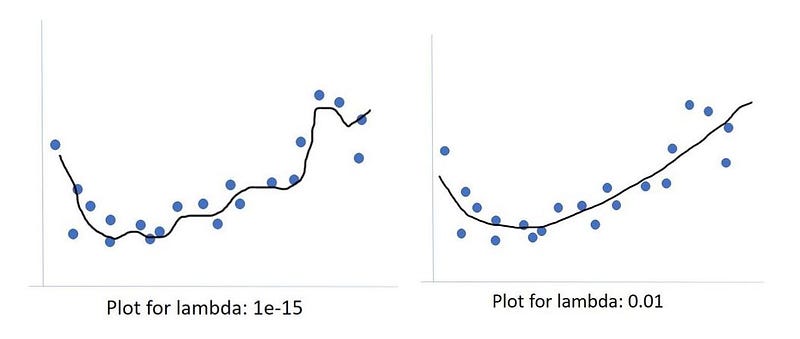
In the example fits above I approximate some form of regression, in this case, probably not a linear regression. And that regression worked pretty well. And then we added the lambda parameter. And hopefully, things got better. If I were to eyeball this here, I would probably want the one on the right. My rationale is, I see these blue dots, they are flying all over the place, they are up and down above and beneath that black line. I expect there to be overall, more variation in where those blue dots can land, a lot of variation. And so I think that trying to find the model that tries to minimize the residuals of these blue dots will try to minimize it too much, what will happen is it will become too complex of a model, it will overfit. And then when new data comes by, data that the model has never seen, that new data is not going to be there where this model is fitting.

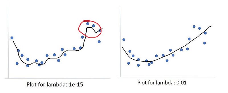
So for instance, this little quirk circled in red, looks pretty good. But my guess is that is just because one or two data points had these high y values relatively - high y values. Methinks that was just a quirk. Probably this should just go straight over, as it does on the right-most image. Because if I look at how much overall these blue points are going up and down, I cannot really justify creating a model that is trying to go down to catch to minimize the residual of this one bluepoint and then going right back up. As such, the small lambda value is likely overfitting and I believe that the 1/100 lambda value on the right actually fits the data much better and will generalize better.

LASSO

LASSO regression does pretty much the same thing; it is another way to limit the number of independent variables in the regression. The only difference is, it uses the absolute value. Now the thing is that because of the math, what it does is not just reduce the coefficients, LASSO actually removes the coefficients. Many people like LASSO for this reason: the coefficients can actually go to zero, whereas in the Ridge regression, they do not go to zero, they become small, but they never vanish.

Now, you can always help the last way, if you see that coefficient has gotten really small, you can just say, “Okay, I’m going to just toss this column, because it has such a small coefficient.” What is nice about LASSO is that it will actually do that for you in an intelligent way.

Beta a vector of your coefficients. Instead of squaring them, you just take the absolute value.

Linear algebra

Next is a quick review of linear algebra. Why do we have a quick review of linear algebra? Well, because machine learning is a lot of linear algebra and the more you understand about the machine learning algorithms, the often the better you can apply them. When studying data science, you are not studying machine learning, you are studying how to use the machine learning algorithms.

Algebraic properties of matrices:

• add/subtract matrices: must be of the same dimensions (m * n)
• for multiplication of matrices: inner dimensions must match
• remember that matrix multiplication is not commutative: A x B != B x A
• a matrix multiplied by its inverse yields the identity matrix
• matrix division is not defined

Linear regression with matrices

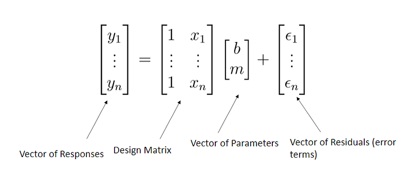
Consider the linear regression formula:

written as a matrix:

which can be rewritten as:

For linear regression with matrices, if you have, say 10 cases, that means 10 points and you will have 10 columns, then there will be an exact, best solution. There will be a simple solution to that. However, not in every case, there are cases where you have colinearity, which means when one column is basically the same as another column or the same as a combination of some other columns. When this occurs you generally have infinitely many solutions. And we do not like this because having infinitely many solutions, means you do not have any useful solutions. If then there are situations where there is simply no solution can occur. But the general case or the case that you hope for is that you have exactly one good solution.

Most of the time, when we do machine learning, or data science is we have many more cases than we have variables; we have many more data points than we have columns; we have many more rows than we have columns — I am just repeating the same thing over and over with slightly different words. This is going to cause us an issue, for one thing, that means our matrix of x is not a square matrix.

So when we want to invert it, and I will show you that we will want to do that, it is going to cause us some problems, along with colinearity and stuff like that.

These concepts are best demonstrated in code.

Python example: Singular value decomposition

Previously, I mentioned stepwise regression as a way to regularize, by finding meaningful features one at a time, either by the forward or backward methodology. I now introduce singular value decomposition (SVD) as another meaningful way to find features.

Regularization methods stabilize the inverse of the model matrix. We will use the SVD method to stabilize a model matrix.

N.B: Stepwise regression is a computationally-intensive process since we must recompute the model many times. There are methods that allow computation of the updated model, but with a large number of features, there are numerous permutations. We need methods that can handle hundreds, thousands, or even millions of features. Consider a small data set with only 20 features. The amount of possible linear models with NO interaction terms is given by:

Which is the sum of the 21st row of Pascal’s triangle. This comes out to be:

Although according to our algorithm, this would be the maximum number of models to compute, you can see how computationally hard this becomes when naively considering stepwise regression.

In order to understand the motivation and methods of feature selection/transformation, I will review some linear algebra.

Linear algebra review

import numpy as np

a_list = [2]*3
print(a_list)
print(type(a_list))
a = np.array([2]*3)
print(a)
print(type(a))
b = np.arange(1, 4)
print(b)
print(type(b))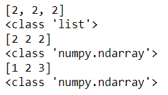

Matrix multiplication and addition

a2d = np.array([[2]*3, [3]*3])
print(‘a: \n{} \n a-size: {}’.format(a2d, a2d.shape))
b2d = np.reshape(np.arange(1,7), newshape=(2, 3))
print(‘\nb: \n{} \n b-size: {}’.format(b2d, b2d.shape))

# Addition
print(‘\nAddition: \n {}’.format(a2d + b2d))
# Multiplication
print(‘\nMultiplication: \n {}’.format(a2d * b2d))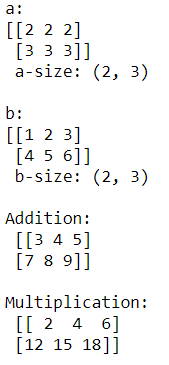

Matrix transposition

We can also transpose a two-dimensional matrix by flipping the rows and columns. We use the numpy method np.transpose.

print(‘Try transposing on a vector…’)
print(np.transpose(a))
# Transposition on a vector does not work

print(‘Now reshape a into 2D and then transpose:’)
print(np.transpose(np.reshape(a, newshape=(1,3))))
print(‘Now transpose a 2d matrix:’)
print(np.transpose(a2d))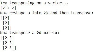

Matrix dot product

We need to know how to compute the dot product, which is also known as the scalar product or inner product of two vectors of equal length, via element-wise multiplication then summing them all up:

print(‘np.dot(a, b) = np.dot({}, {})’.format(a, b))
np.dot(a, b)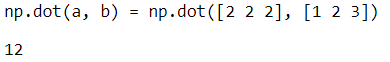

The square root of the inner product of a vector with itself is the length or L2 norm of the vector:

We can also write the inner product as:

aa = np.array([1, 0, 0])
bb = np.array([0, 1, 1])
print(inner_prod(aa, bb))

Here are some operations on matrices. Let A and B be m=4 rows by n=3 columns matrices:

A = np.array([[4]*3]*4) 
print(A)
B = np.array(np.reshape(np.arange(1, 13), newshape = (4, 3)))
print(B)
C = np.array(np.reshape(np.arange(1, 9), newshape = (4, 2)))
print(C)
np.dot(np.transpose(A), C)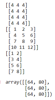

Identity matrix

This special, square matrix has ones on the diagonal and zeros elsewhere:

The identity multiplied by any matrix gives that matrix. If AB is a rectangular matrix then:

In numpy the Identity matrix is called np.eye and takes as an argument the number of rows/columns:

I3 = np.eye(3)
I4 = np.eye(4)

print(‘I (3X3) = \n{}’.format(I3))
print(np.dot(I3, AtB))

print(‘I (4x4) = \n{}’.format(I4))
print(np.dot(I4, ABt))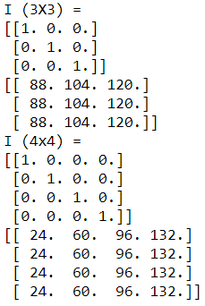

Inverse of a matrix

Define and compute an inverse of a matrix such that:

Use the Linear Algebra methods in numpy to get the inverse of matrix M with np.linalg.inv

M = np.array([[1., 4.], [-3., 2.]])
M_inverse = np.linalg.inv(M)

print(‘M: \n{}’.format(M))
print(‘\nM_inv = \n{}’.format(M_inverse))
print(‘\nM_inv * M = \n{}’.format(np.dot(M_inverse, M)))
print(‘\nM * M_inv = \n{}’.format(np.dot(M, M_inverse)))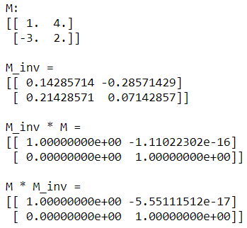

With this brief refresher aside, we can now jump into regularizing models with SVD.

Singular Value Decomposition

In machine learning, we often encounter matrices that cannot be inverted directly. Instead, we need a decomposition of A that allows us to compute A^−1, which we can do with SVD:

• U is the orthogonal unit norm left singular vectors
• V is the orthogonal unit norm right singular vectors, and V∗ is the conjugate transpose; for real-valued A this is just VT
• D is a diagonal matrix of singular values, which are said to define a spectrum
• A is comprised of the linear combination of singular vectors scaled by singular values

To compute the SVD of a matrix and view the results execute the code in the cell below. We use the numpy method called np.linalg.svd using s for the singular values:

U, s, V = np.linalg.svd(B, full_matrices=False)
print(‘B: {}’.format(B)) # ESHx
print(‘U: {}’.format(U))
print(‘s: {}’.format(s))
print(‘V: {}’.format(V))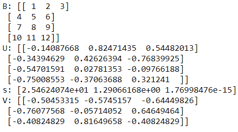

Regularization with Ridge and Lasso Regression

So far, we have looked at two approaches for dealing with over-parameterized models; feature selection by stepwise regression and singular value decomposition. In this section, we will explore the most widely used regularization method for optimization-based machine learning models, Ridge regression.

Let’s start by examining the matrix-equation formulation of the linear regression problem. The goal is to compute a vector of model coefficients or weights which minimize the mean squared residuals, given a vector of data 𝑥x and a model matrix A. We can express our model as:

Execute the code in the cell below which computes the (𝐴^𝑇 * 𝐴+𝜆²)^-1 * A^T matrix with a lambda value of 0.1

U, s, V = np.linalg.svd(M, full_matrices=False)

# Calculate the inverse singular value matrix from SVD
lambda_val = 1.0
d = np.diag(1. / (s + lambda_val))

print(‘Inverse Singular Value Matrix:’)
print(d)

# Compute pseudo-inverse
mInv = np.dot(np.transpose(V), np.dot(d, np.transpose(U)))

print(‘M Inverse’)
print(mInv)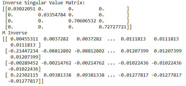

Bias-variance trade-off

The bias-variance trade-off is a fundamental property of machine learning models. To understand this trade-off let’s decompose the mean square error for a model as follows:

Regularization will reduce variance, but increases bias. Regularization parameters are chosen to minimize delta_X. In many cases, this process proves challenging, involving significant time-consuming trial and error.

The irreducible error is the limit of model accuracy. Even if you had a perfect model with no bias or variance, the irreducible error is inherent in the data and model. You cannot do better.

The statsmodels package allows us to compute a sequence of Ridge regression solutions. The function that does this uses a method called ‘Elasticnet’, know that ridge regression is a specific case of elastic-net, and I will talk more about this later.

N.B: This is a continuation of my previous work on the Galton family dataset.

The code in the cell below computes solutions for 20 values of lambda:

# Ridge regression with various penalties in Statsmodels
# sequence of lambdas
log_lambda_seq = np.linspace(-6, 2, 50)
lambda_seq = np.exp(log_lambda_seq)

coeffs_array = []
rsq_array = []
formula = ‘childHeight ~ mother + father + mother_sqr + father_sqr + 1’

for lamb in lambda_seq:
 ridge_model = sm.ols(formula, data=male_df).fit_regularized(method=’elastic_net’, alpha=lamb, L1_wt=0)
 coeffs_array.append(list(ridge_model.params))
 predictions = ridge_model.fittedvalues
 residuals = [x — y for x, y in zip(np.squeeze(predictions), childHeight)]

SSR = np.sum(np.square(residuals))
 SST = np.sum(np.square(childHeight — np.mean(childHeight)))

rsq = 1 — (SSR / SST) 
 rsq_array.append(rsq)

# pull out partial slopes (drop intercept version)
beta_coeffs = [x[1:] for x in coeffs_array]
plt.plot(log_lambda_seq, beta_coeffs)
plt.title(‘Partial Slopes vs Log-Lambda’)
plt.ylabel(‘Partial Slope Values’)
plt.xlabel(‘Log-Lambda’)
plt.show()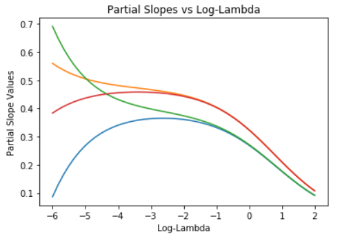

Plot partial slopes vs R²:

# % deviance explained
plt.plot(rsq_array, beta_coeffs)
plt.xlim([0.0, 0.25])
plt.title(‘Partial Slopes vs Log-Lambda’)
plt.xlabel(‘R-squared’)
plt.ylabel(‘Partial Slopes’)
plt.show()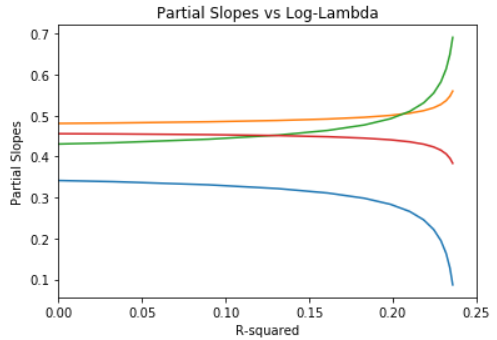

Notice that as lambda increases, the values of the 4 model coefficients decrease toward zero. When all coefficients are zero, the model predicts all values of the label as zero! In other words, high values of lambda give highly biased solutions, but with very low variance.

For small values of lambda, the situation is just the opposite. The solution has a low bias, but is quite unstable, having maximum variance. This bias-variance trade-off is a key concept in machine learning.

LASSO regression

We can also do regularization using other norms. LASSO or L1 regularization limits the sum of the absolute values of the model coefficients. The L1 norm is sometimes known as the Manhattan norm since distances are measured as if you were traveling on a rectangular grid of streets.

You can also think of LASSO regression as limiting the L1 norm of the values of the model coefficient vector. The value of lambda determines how much the norm of the coefficient vector constrains the solution.

Performing the same calculations as before, but with a different regularization norm and associated penalty:

# LASSO regression with a sequence of lambdas
# sequence of lambdas
log_lambda_seq = np.linspace(-6, 2, 50)
lambda_seq = np.exp(log_lambda_seq)

coeffs_array = []
rsq_array = []
formula = ‘childHeight ~ mother + father + mother_sqr + father_sqr + 1’

for lamb in lambda_seq:
 ridge_model = sm.ols(formula, data=male_df).fit_regularized(method=’elastic_net’, alpha=lamb, L1_wt=1)
 coeffs_array.append(list(ridge_model.params))
 predictions = ridge_model.fittedvalues
 residuals = [x — y for x, y in zip(np.squeeze(predictions), childHeight)]

SSR = np.sum(np.square(residuals))
 SST = np.sum(np.square(childHeight — np.mean(childHeight)))

rsq = 1 — (SSR / SST)
 rsq_array.append(rsq)

# drop intercept version
beta_coeffs = [x[1:] for x in coeffs_array]
plt.plot(log_lambda_seq, beta_coeffs)
plt.title(‘Partial Slopes vs Log-Lambda’)
plt.ylabel(‘Partial Slope Values’)
plt.xlabel(‘Log-Lambda’)
plt.show()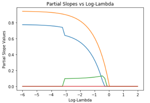

# plot partial slopes vs R squared (% deviance explained)
plt.plot(rsq_array, beta_coeffs)
plt.xlim([0.0, 0.25])
plt.title(‘Partial Slopes vs Log-Lambda’)
plt.xlabel(‘R-squared’)
plt.ylabel(‘Partial Slopes’)
plt.show()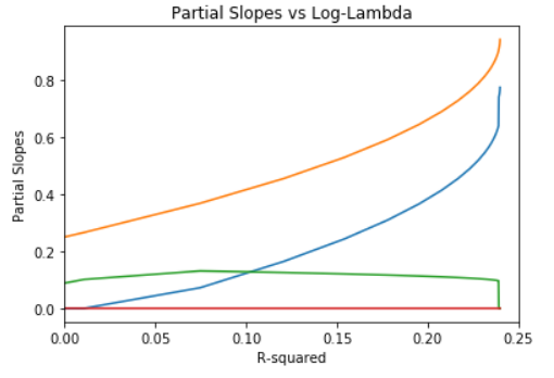

Notice that model coefficients are much more tightly constrained than for L2 regularization. In fact, only two of the possible model coefficients have non-zero values at all! This is typical of L1 or LASSO regression.

Elastic Net regression

The elastic net algorithm uses a weighted combination of L1 and L2 regularization. As you can probably see, the same function is used for LASSO and Ridge regression with only the L1_wt argument changing. This argument determines how much weight goes to the L1-norm of the partial slopes. If the regularization is pure L2 (Ridge) and if L1_wt = 1.0 the regularization is pure L1 (LASSO).

The code in the cell below gives equal weight to each regression method. Execute this code and examine the results:

# ElasticNet Regression with a sequence of lambdas
# sequence of lambdas
log_lambda_seq = np.linspace(-6, 0, 50)
lambda_seq = np.exp(log_lambda_seq)

coeffs_array = []
rsq_array = []
formula = ‘childHeight ~ mother + father + mother_sqr + father_sqr + 1’

for lamb in lambda_seq:
 ridge_model = sm.ols(formula, data=male_df).fit_regularized(method=’elastic_net’, alpha=lamb, L1_wt=0.75)
 coeffs_array.append(list(ridge_model.params))
 predictions = ridge_model.fittedvalues
 residuals = [x — y for x, y in zip(np.squeeze(predictions), childHeight)]

SSR = np.sum(np.square(residuals))
 SST = np.sum(np.square(childHeight — np.mean(childHeight)))

rsq = 1 — (SSR / SST)
 rsq_array.append(rsq)

# pull out partial slopes (drop intercept version)
beta_coeffs = [x[1:] for x in coeffs_array]
plt.plot(log_lambda_seq, beta_coeffs)
plt.title(‘Partial Slopes vs Log-Lambda’)
plt.ylabel(‘Partial Slope Values’)
plt.xlabel(‘Log-Lambda’)
plt.show()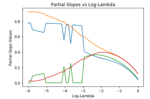

# plot partial slopes vs R squared (% deviance explained)
plt.plot(rsq_array, beta_coeffs)
plt.xlim([0.0, 0.25])
plt.title(‘Partial Slopes vs Log-Lambda’)
plt.xlabel(‘R-squared’)
plt.ylabel(‘Partial Slopes’)
plt.show()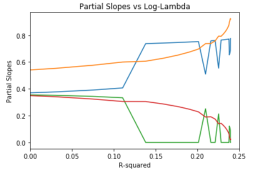

Notice that the elastic net model combines some of the behaviors of both L2 and L1 regularization.

Conclusion

In this article and last week’s I looked at 3 methods as a solution to the problem of overfitting models:

• Stepwise Regression to eliminate features one at a time
• Singular Value Decomposition to find meaningful features
• Lasso, Ridge, and ElasticNet Regularization to stabilize over-parameterized models

Important terms include:

• AIC — the model log-likelihood adjusted for the number of model parameters
• Deviance — a measure of the relative likelihood of the model (a generalization of variance)
• SVD — Singular Value Decomposition describes a matrix as a linear combination of a series of vectors U, V, D
• Singular values s — the diagonal matrix of singular values used as a scaling term
• Lambda — a small bias term added to singular values to stabilize the inverse singular value matrix
• PCA — Principal Component Analysis to determine what new features can be made from linear combinations that are independent of each other by using functions and the SVD
• PCR — Principal Component Regression uses the PCA to perform a “regularized” regression
• L1 regularization — LASSO regularization using the “Manhattan” norm
• L2 Norm regularization — Ridge regularization limiting the “Euclidean” norm of values of the model coefficient vector
• ElasticNet algorithm — a weighted combination of L1 and L2 regularization

And I briefly reviewed linear algebra operations:

• Adding vectors and matrices
• Multiplying vectors and matrices
• Transposing matrices with np.transpose
• Dot product or scalar product or inner product with np.dot
• L2 norm of a vector
• Identity matrix with np.eye
• Inverse of a matrix with np.linalg.inv
• Singular value decomposition with np.linalg.svd
• Creating a diagonal matrix with np.diag

Up to now, I have been working strictly with linear regression models. Next, I will look at a widely used variation on the linear model know as logistic regression!

Find me on Linkedin

Physicist cum Data Scientist- Available for new opportunity | SaaS | Sports | Start-ups | Scale-ups