
Research Paper Review: A comparison between ARIMA, LSTM, and GRU for time series forecasting

Since I spend much of my time on Kaggle, I don’t get a lot of opportunities to focus on time series forecasting, but I decided to study it as it relates to Tensorflow. Tensorflow, developed by Google, is Python’s library that creates neural networks. In addition to making predictions on tabular data, images, natural language, and even sound, Tensorflow can also make predictions on time series data.
I found a research paper that I would have liked to have read in its entirety, but only the abstract and references were made public on the internet. The research paper was titled, ‘A Comparison between ARIMA, LSTM and GRU for Time Series Forecasting’, and was published for the 2019 2nd International Conference on Algorithms, Computing, and Artificial Intelligence. The abstract of the paper can be found here:- https://dl.acm.org/doi/abs/10.1145/3377713.3377722
The abstract of the piece stated (in paraphrase) that the authors compared three different models to make time series forecasts on a Bitcoin price dataset. The Bitcoin dataset can be downloaded from Yahoo!, and it can be found here:- https://finance.yahoo.com/quote/BTC-USD/history/
The three models that the authors of the paper used in the research study they carried out were ARIMA, LSTM and GRU. The result of the research these individuals carried out was that ARIMA had a lower root mean squared error (RMSE), which means that it outperformed LSTM and GRU.
Time series forecasting is well within my capabilities, so I decided to make an attempt at replicating their work, which I was not able to obtain freely on the internet. After I carried out my research, which I hope was in parallel with the authors of the paper, I found that the results I achieved were different, with GRU outperforming LSTM and ARIMA.
ARIMA
Statsmodels’ ARIMA (AutoRegressive Integrated Moving Average) is a popular time series modelling technique implemented in the statsmodels library, which is a Python package for statistical modelling and analysis. ARIMA models are widely used for forecasting and analysing time series data.
The ARIMA model combines three components: autoregressive (AR), differencing (I), and moving average (MA).
- Autoregressive (AR): This component models the relationship between an observation and a certain number of lagged observations (past values). It assumes that the current value of the time series is linearly dependent on its previous values.
- Differencing (I): This component handles non-stationary data by differencing the time series. It subtracts the previous observation from the current observation, which helps remove trends or seasonality in the data.
- Moving Average (MA): This component models the dependency between an observation and a residual error from a moving average of the lagged observations. It assumes that the current value of the time series is related to the weighted average of its past errors.
The notation used for an ARIMA model is ARIMA(p, d, q), where:
- p represents the order of the autoregressive component, indicating the number of lagged observations to consider.
- d represents the degree of differencing, indicating the number of times the data needs to be differenced to achieve stationarity.
- q represents the order of the moving average component, indicating the number of lagged residuals to consider.
Overall, the ARIMA model in statsmodels is a powerful tool for time series analysis and forecasting, providing a flexible framework for modelling and predicting various types of time-dependent data.
GRU
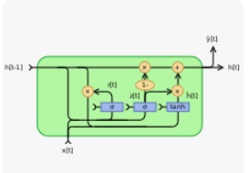
TensorFlow’s Gated Recurrent Unit (GRU) is a type of recurrent neural network (RNN) architecture that is designed to capture dependencies and patterns in sequential data. It is a variation of the traditional RNN and offers an improvement over the vanishing gradient problem and the difficulty of capturing long-term dependencies.
The GRU consists of recurrent units that operate over a sequence of inputs. Each recurrent unit within the GRU has a gating mechanism that controls the flow of information. The main components of the GRU are as follows:-
- Update Gate: The update gate controls how much of the previous hidden state should be retained and combined with the current input. It determines the amount of information to forget or remember from the past.
- Reset Gate: The reset gate helps the GRU decide how much of the previous hidden state should be ignored. It allows the network to selectively reset or update parts of the hidden state based on the current input.
- Candidate Activation: The candidate activation calculates a new candidate hidden state based on the current input and the previous hidden state. It combines information from the input and the reset gate to determine the potential new state.
- Hidden State: The hidden state represents the memory of the GRU. It stores the learned information from previous inputs and is updated based on the input, the reset gate, and the update gate.
The GRU architecture allows for capturing short-term dependencies effectively, and its gating mechanism enables the model to control the flow of information and adapt to different time scales within the data. It has been widely used in various sequence-based tasks, including natural language processing, speech recognition, and time series analysis.
LSTM
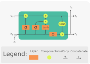
TensorFlow’s Long Short-Term Memory (LSTM) is a type of recurrent neural network (RNN) architecture designed to address the limitations of traditional RNNs, such as the vanishing gradient problem and the difficulty of capturing long-term dependencies in sequential data.
LSTM networks consist of memory cells that allow information to persist over long sequences, enabling them to capture and remember long-term dependencies. The main components of an LSTM cell are as follows:
- Cell State ©: The cell state serves as the memory of the LSTM. It runs linearly through the entire sequence and can retain or forget information. The cell state can be thought of as a conveyor belt that runs through the LSTM, allowing information to flow while being modified by gates.
- Input Gate (i): The input gate determines how much new information should be stored in the cell state. It controls the update of the cell state based on the current input and the previous hidden state.
- Forget Gate (f): The forget gate decides what information should be discarded from the cell state. It regulates the flow of information from the previous cell state to the current cell state. It is used to forget irrelevant information from previous time steps.
- Output Gate (o): The output gate determines how much of the current cell state should be exposed as the output. It controls the amount of information that is sent to the next hidden state and ultimately to the output of the LSTM.
- Hidden State (h): The hidden state is the output of the LSTM at a particular time step. It carries information that is selectively propagated to subsequent time steps.
The LSTM’s architecture and gating mechanisms allow it to capture and retain information over long sequences, making it particularly effective for tasks that involve modelling long-term dependencies, such as natural language processing, speech recognition, and time series analysis.
Coding
I prepared the computer programs using Google Colab, which is a free online Jupyter Notebook hosted by Google. Google Colab is a great platform to use, with the one exception that it does not have a sufficient undo function, so care needs to be taken not to accidentally overwrite or delete valuable code.
For the programs, I imported all of the standard libraries that are needed to execute the programs, such as pandas, numpy, sklearn, statsmodels, scipy, sklearn, tensorflow, matplotlib, and seaborn.
I downloaded the Bitcoin csv file into my Google drive, where it was stored for use in the two programs that I created for this review.
Code for ARIMA using Statsmodels
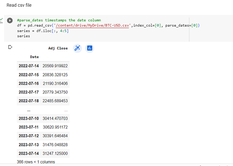
Once the standard libraries that I would need were imported, I used pandas to read the csv file in, making the date column the index, and parsing the dates. I used only the 4th column of the dataframe as the univariate time series data:-
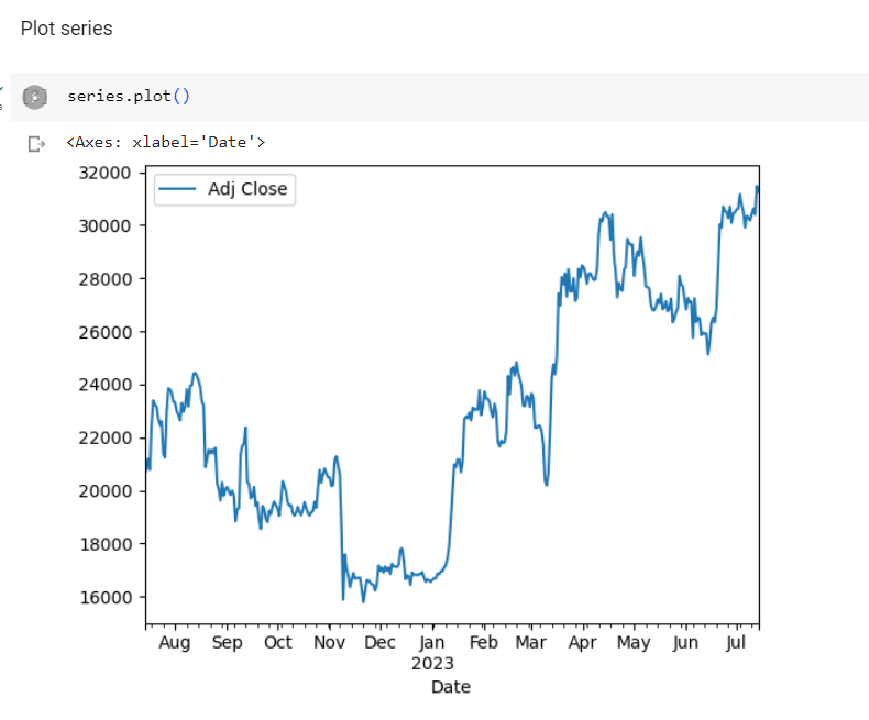
I used matplotlib to visualise the time series:-
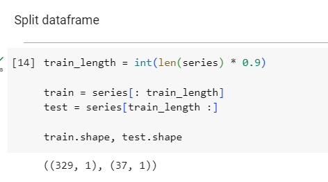
I split the dataframe into train and test sets:-
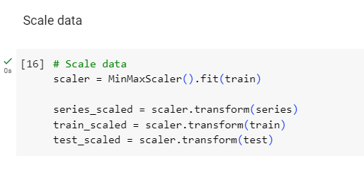
I used sklearn’s MinMaxScaler to scale the data from 0 to 1:-
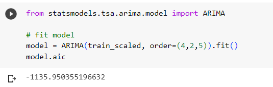
I used statsmodels’ ARIMA model to train the data:-
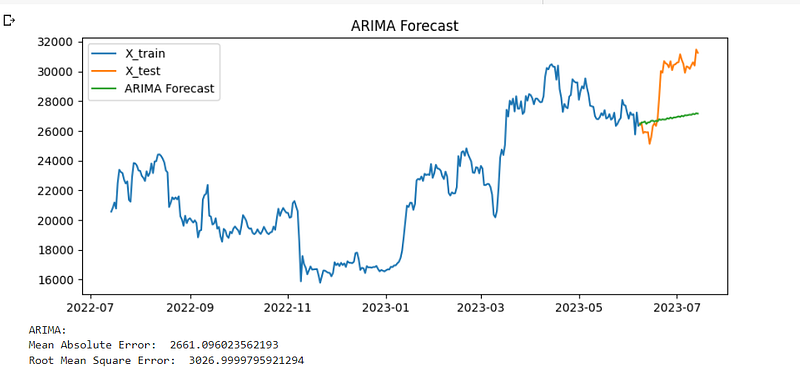
I made predictions on the test set, plotted it onto a graph, and obtained the root mean squared error (RMSE) of 3027:-
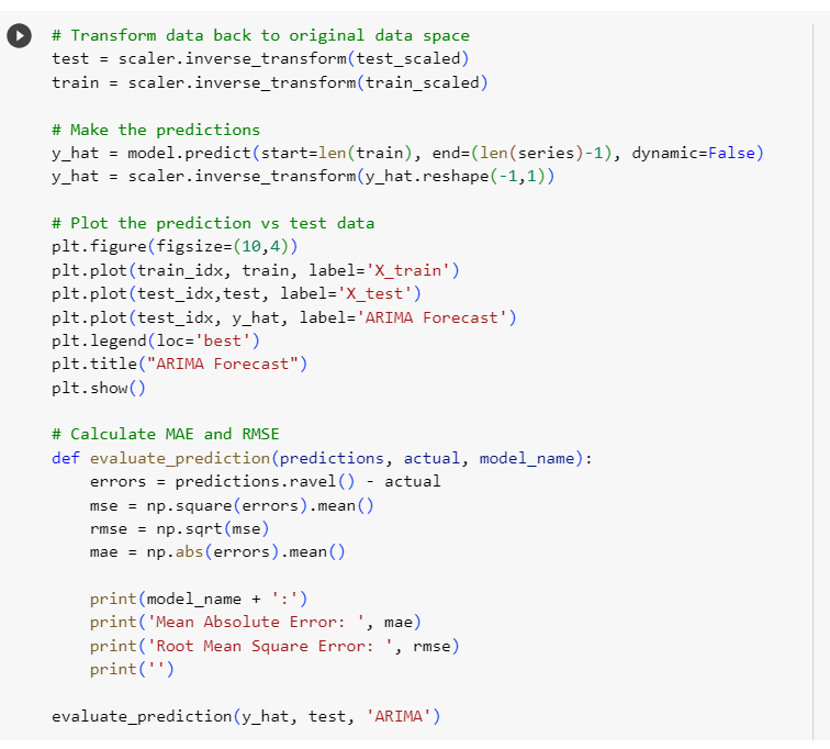
Below is a plot of the train set, test set, and predictions:-
Code for GRU and LSTM in Tensorflow
I read the dataset, converted it to a dataframe, and visualised it in the same manner that I had previously done when I made predictions using statsmodels’ ARIMA model.
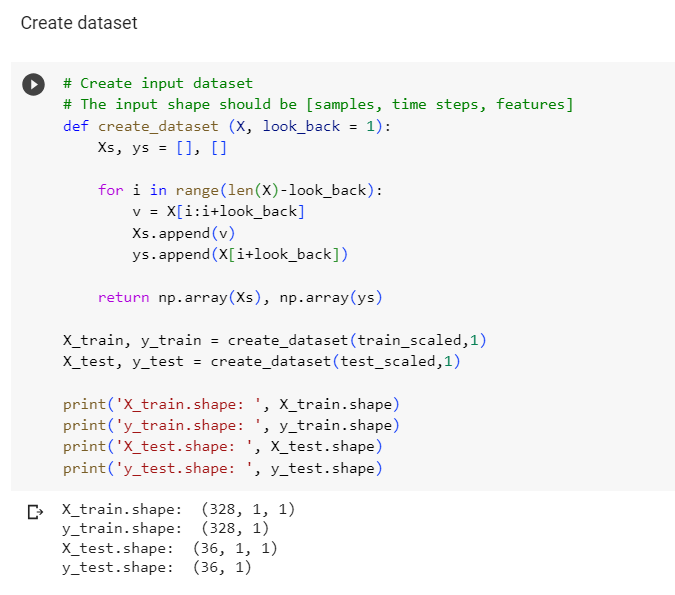
Because the GRU and LSTM models are neural networks, I had to create an input dataset, as seen below:-
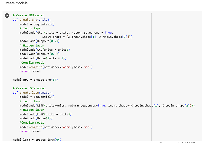
I then created the GRU and LSTM models and compiled them:-
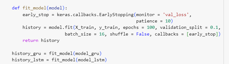
I trained the models:-
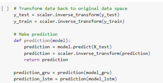
I then made predictions on the models:-
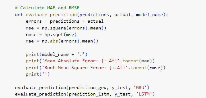
I calculated the root mean squared error (RMSE) of the two models:-
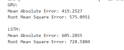
The RMSE for the GRU was 575, which performed better than LSTM and ARIMA:-
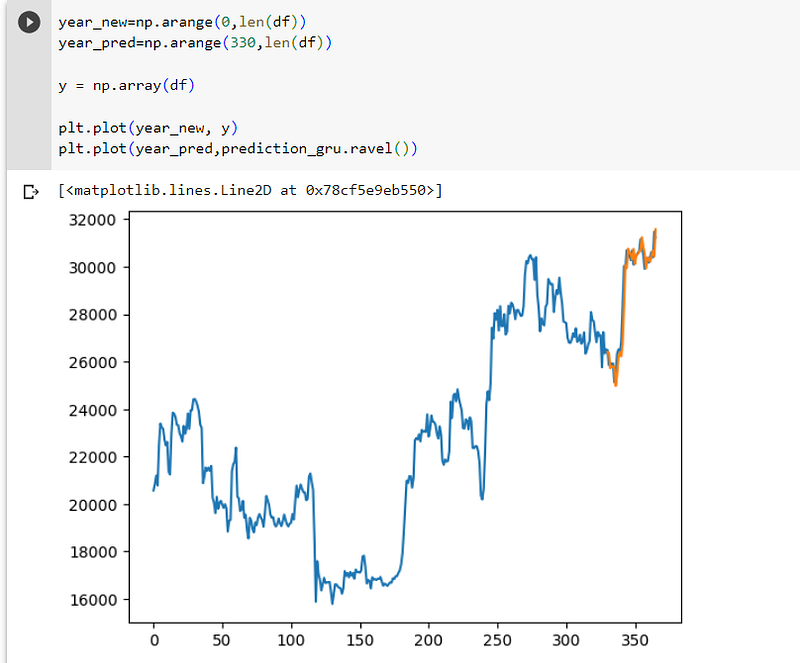
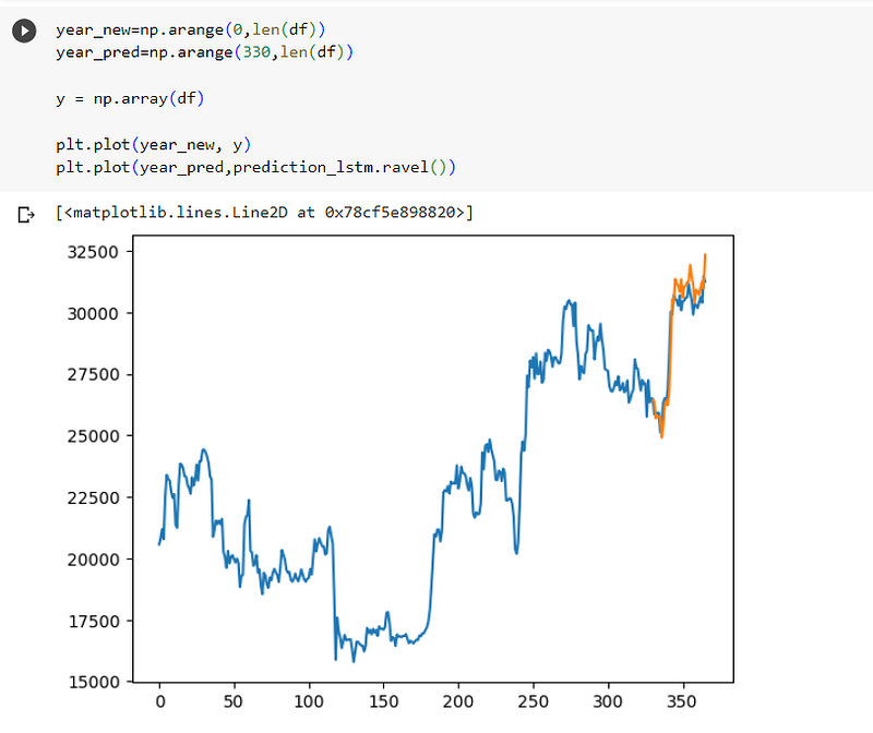
I then used matplotlib to visualise both the GRU and LSTM models:-
Conclusion
Because the content of the research paper was not made freely available on the internet, I carried out research of my own based on a dataset on Bitcoins from Yahoo! financial page. I employed the three models that the authors of the paper used, being ARIMA, GRU and LSTM. My findings were different, however, as GRU outperformed ARIMA and LSTM.
I have prepared a code review to accompany this blog post, and it can be viewed here:- https://youtu.be/e5T8oBhywhA


