
Reproducing Dynamic Mode Decomposition on Fluid Flow Data in Python
What is the fluid flow data? How to visualize these data? How to reproduce dynamic mode decomposition in Python?
Dynamic mode decomposition (DMD) is a data-driven dimensionality reduction approach for discovering underlying data patterns of time series [1–3]. Its introduction into spatiotemporal data analysis shows great potential, and one important application of DMD is analyzing fluid dynamics. In our previous blog post [4], we discussed how to reproduce DMD in the case of multivariate time series forecasting. Today, we introduce how to reproduce DMD on the fluid flow data with NumPy in Python. Let’s get started!
Fluid Flow Data
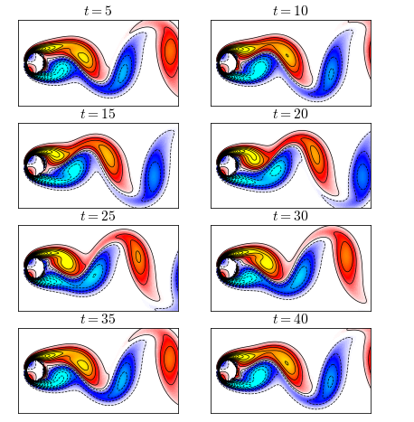
In this story, we consider the cylinder wake dataset (source: http://dmdbook.com/) for analysis. The dataset is collected from the fluid flow passing a circular cylinder. This is a representative three-dimensional flow dataset in fluid dynamics, which consists of matrix-variate time series of vorticity field snapshots for the wake behind a cylinder. The dataset is of size 199-by-449-by-150, and the last dimension refers to 199-by-449 vorticity fields with 150 time snapshots.
In the following analysis, we reshape the data as multivariate time series matrix of size 89,351-by-150, which seems to be high-dimensional. To design a toy example, we only use the first 50 snapshots. We draw some snapshots of the dataset as shown in Figure 1.
To reproduce Figure 1 in Python, please consider the following codes.
import numpy as np
import seaborn as sns
import scipy.io
import matplotlib.pyplot as plt
from matplotlib.colors import ListedColormap, LinearSegmentedColormap
color = scipy.io.loadmat('CCcool.mat')
cc = color['CC']
newcmp = LinearSegmentedColormap.from_list('', cc)
dense_tensor = np.load('tensor.npz')['arr_0']
dense_tensor = dense_tensor[:, :, : 50]
M, N, T = dense_tensor.shapeplt.rcParams['font.size'] = 13
plt.rcParams['mathtext.fontset'] = 'cm'
fig = plt.figure(figsize = (7, 8))
id = np.array([5, 10, 15, 20, 25, 30, 35, 40])
for t in range(8):
ax = fig.add_subplot(4, 2, t + 1)
ax = sns.heatmap(dense_tensor[:, :, id[t] - 1], cmap = newcmp, vmin = -5, vmax = 5, cbar = False)
ax.contour(np.linspace(0, N, N), np.linspace(0, M, M), dense_tensor[:, :, id[t] - 1], levels = np.linspace(0.15, 15, 30), colors = 'k', linewidths = 0.7)
ax.contour(np.linspace(0, N, N), np.linspace(0, M, M), dense_tensor[:, :, id[t] - 1], levels = np.linspace(-15, -0.15, 30), colors = 'k', linestyles = 'dashed', linewidths = 0.7)
plt.xticks([])
plt.yticks([])
plt.title(r'$t = {}$'.format(id[t]))
for _, spine in ax.spines.items():
spine.set_visible(True)
plt.show()Note that we place the fluid data at our GitHub repository: https://github.com/xinychen/fluid-inpainting.
DMD Model
In our previous blog post [5], we discussed the detailed algorithm of DMD. In this story, we use the Python codes of DMD in that blog post for introducing this story. The function of DMD is given as here:
import numpy as npdef DMD(data, r):
"""Dynamic Mode Decomposition (DMD) algorithm."""
## Build data matrices
X1 = data[:, : -1]
X2 = data[:, 1 :]
## Perform singular value decomposition on X1
u, s, v = np.linalg.svd(X1, full_matrices = False)
## Compute the Koopman matrix
A_tilde = u[:, : r].conj().T @ X2 @ v[: r, :].conj().T * np.reciprocal(s[: r])
## Perform eigenvalue decomposition on A_tilde
eigval, eigvec = np.linalg.eig(A_tilde)
## Compute the coefficient matrix
Psi = X2 @ v[: r, :].conj().T @ np.diag(np.reciprocal(s[: r])) @ eigvec
return eigval, eigvec, PsiIn the case, r is the predefined low rank of DMD. eigval and eigveccorrespond to the eigenvalues and the eigenvectors of Koopman matrix in DMD. In particular, eigval can be interpreted as DMD spectrum, appearing as complex conjugate pairs. Psi refers to the dynamic modes.
Toy Example on the Fluid Flow Data
In this story, we use the first 50 snapshots of the fluid flow dataset for analysis. We set the rank of DMD as 5.
import numpy as np
import time
dense_tensor = np.load('tensor.npz')['arr_0']
dense_tensor = dense_tensor[:, :, : 50]
M, N, T = dense_tensor.shape
mat = np.reshape(dense_tensor, (M * N, T), order = 'F')rank = 5
eigval, eigvec, Psi = DMD(mat, rank)Eigenvalues
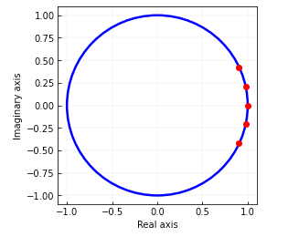
We can check out the eigenvalues (see Figure 2). It seems that all eigenvalues are on the unit circle.
To draw this figure, please try the following Python codes.
import matplotlib.pyplot as pltfig = plt.figure(figsize = (4, 4))
ax = fig.add_subplot(1, 1, 1)
ax.set_aspect('equal', adjustable = 'box')
plt.plot(eigval.real, eigval.imag, 'o', color = 'red', markersize = 6)
circle = plt.Circle((0, 0), 1, color = 'blue', linewidth = 2.5, fill = False)
ax.add_patch(circle)
plt.grid(axis = 'both', linestyle = "--", linewidth = 0.1, color = 'gray')
ax.tick_params(direction = "in")
plt.xlabel('Real axis')
plt.ylabel('Imaginary axis')
plt.show()Spatial Modes
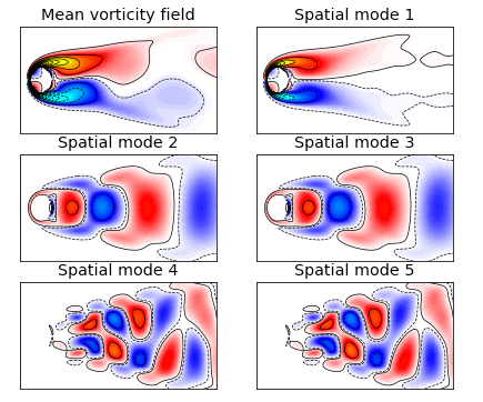
We can also check out the spatial modes, i.e., Psi in the outputs of the DMD function. Figure 3 shows both the mean vorticity field and the spatial modes. Of these results, the spatial mode 1 shows the most basic pattern which is similar to the mean vorticity field. The remaining spatial modes identify the wave pattern of the fluid flow.
To draw this figure, please try the following Python codes.
import seaborn as sns
import scipy.io
import matplotlib.pyplot as plt
from matplotlib.colors import ListedColormap, LinearSegmentedColormap
color = scipy.io.loadmat('CCcool.mat')
cc = color['CC']
newcmp = LinearSegmentedColormap.from_list('', cc)
W = Psi.realplt.rcParams['font.size'] = 12
fig = plt.figure(figsize = (7, 6))
ax = fig.add_subplot(3, 2, 1)
sns.heatmap(np.mean(dense_tensor, axis = 2), cmap = newcmp, vmin = -5, vmax = 5, cbar = False)
ax.contour(np.linspace(0, N, N), np.linspace(0, M, M), np.mean(dense_tensor, axis = 2), levels = np.linspace(0.15, 15, 20), colors = 'k', linewidths = 0.7)
ax.contour(np.linspace(0, N, N), np.linspace(0, M, M), np.mean(dense_tensor, axis = 2), levels = np.linspace(-15, -0.15, 20), colors = 'k', linestyles = 'dashed', linewidths = 0.7)
plt.xticks([])
plt.yticks([])
plt.title('Mean vorticity field')
for _, spine in ax.spines.items():
spine.set_visible(True)
for t in range(5):
ax = fig.add_subplot(3, 2, t + 2)
ax = sns.heatmap(W[:, t].reshape((199, 449), order = 'F'), cmap = newcmp, vmin = -0.03, vmax = 0.03, cbar = False)
num = 10
ax.contour(np.linspace(0, N, N), np.linspace(0, M, M), W[:, t].reshape((199, 449), order = 'F'), levels = np.linspace(0.0005, 0.05, num), colors = 'k', linewidths = 0.7)
ax.contour(np.linspace(0, N, N), np.linspace(0, M, M), W[:, t].reshape((199, 449), order = 'F'), levels = np.linspace(-0.05, -0.0005, num), colors = 'k', linestyles = 'dashed', linewidths = 0.7)
plt.xticks([])
plt.yticks([])
plt.title('Spatial mode {}'.format(t + 1))
for _, spine in ax.spines.items():
spine.set_visible(True)
plt.show()Conclusion
In this story, we introduce what is fluid flow dataset and how to discover the underlying spatial modes from the data through DMD. If you are interested in the detailed algorithm of DMD, please check out our previous blog posts in [4–5].
References
[1] Peter Schmid (2010). Dynamic mode decomposition of numerical and experimental data. Journal of fluid mechanics, 656: 5–28.
[2] Dynamic mode decomposition on Wikipedia: https://en.wikipedia.org/wiki/Dynamic_mode_decomposition
[3] J. Nathan Kutz, Steven L. Brunton, Bingni W. Brunton, Joshua L. Proctor (2016). Dynamic mode decomposition: Data-driven modeling of complex systems. SIAM.
[4] Dynamic mode decomposition for multivariate time series forecasting. https://readmedium.com/415d30086b4b
[5] Dynamic Mode Decomposition for Spatiotemporal Traffic Speed Time Series in Seattle Freeway. https://towardsdatascience.com/dynamic-mode-decomposition-for-spatiotemporal-traffic-speed-time-series-in-seattle-freeway-b0ba97e81c2c