Replicating Minecraft World Generation in Python

Using Voronoi diagrams and a lot of Perlin/Simplex noise

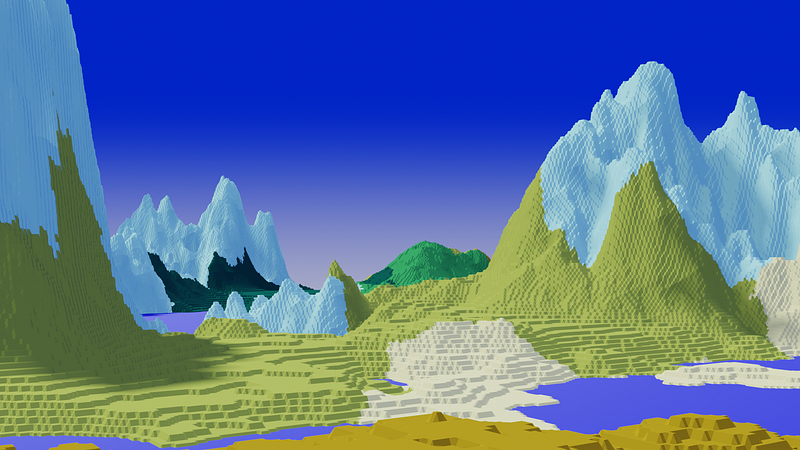
Minecraft, the best-selling game of all time, best known for its pixelated building blocks and infinite worlds, has an amazing procedurally generated terrain with caves, waters, and even different biomes.

Procedural generation is an important part of computer graphics. It is used mostly in video games or in movies. It helps generate random structures that do not have a “machine-like” feeling to them.

Similarly, procedural generation plays an important role in machine learning. It can help generate data that is hard to collect. Training machine learning models requires huge datasets that can be difficult and costly to gather and process. Generating data procedurally can be easily adapted to the exact type of data needed.

I used to play Minecraft as a kid and I always wondered how does it generate never-ending worlds. In this article, I am going to try to replicate this in Python.

Definitions And Limits

We first have to define how our world will be generated.

The world is 3-dimensional, discrete (comprised of blocks of unit size), bounded in the z-axis by 0 and 255, and unbounded is the x and y-axis.
The world contains biomes, each spanning large horizontal areas, that define the nature of the space that the biome occupies.
The world contains rivers, lakes, and oceans.

Every world is defined by a seed. The same seed will always generate the same world.

Generating Worlds

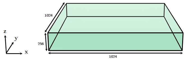
To make the generation process easy, we will divide our world into chunks. Every chunk will occupy a space of 1024×1024×256 blocks.

Every chunk is generated separately. This will help us save, load the world, and generate more parts of the world easily.

Biomes Borders

The first thing we have to do is divide our world into cells on the x and y-axis, each of a certain biome. We will assign to every cell a point representing its center.

Voronoi Diagram

A Voronoi diagram will help us divide our world into cells given a set of points. The main idea behind Voronoi diagrams is that the cell a point belongs to is the cell whose center is the closest.

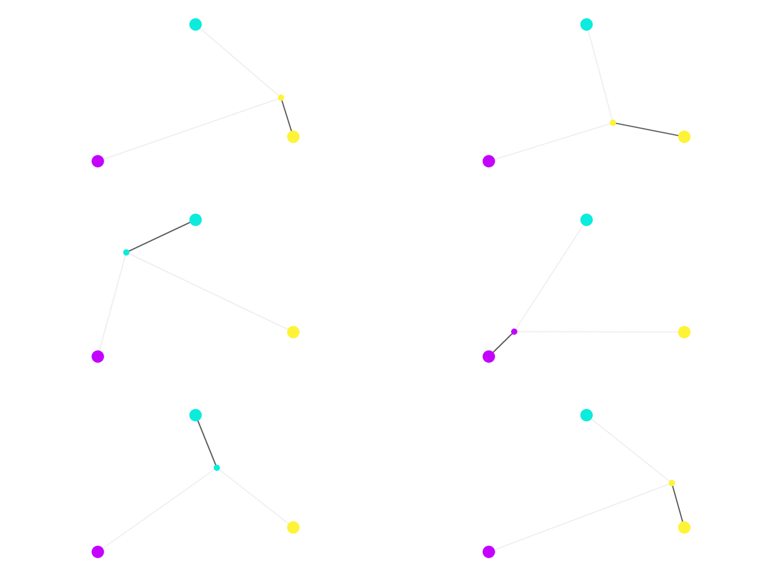
The moving point is colored by the color of the closest point to it. Image by Author.

We can do this for every point in the xy-plane to get the Voronoi diagram of these 3 points.

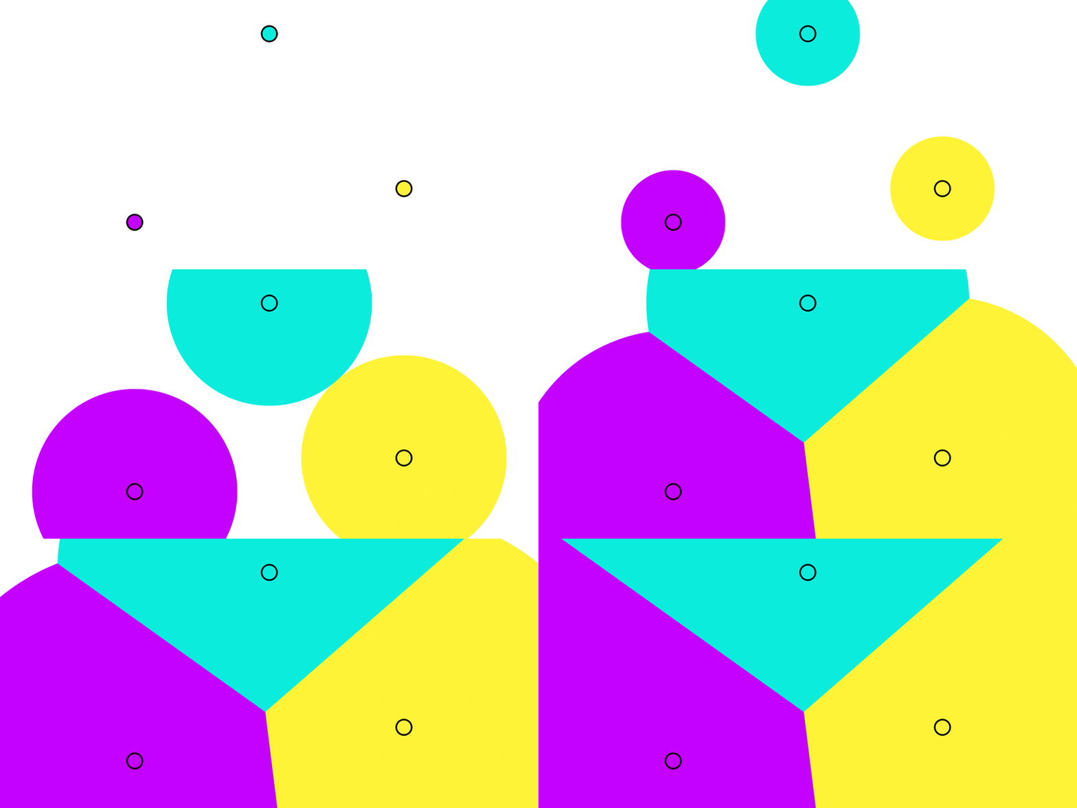
Voronoi diagram of 3 points, animated. Image by Author

Altough this method works, it is painfully slow, especially when the number of points is large.

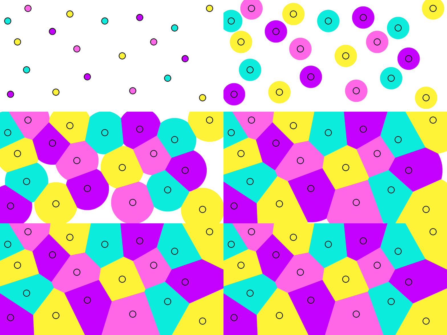
Voronoi diagram of 20 points, animated. Image by Author.

In Python, scipy.spatial has a class called Voronoi that calculates Voronoi diagrams more efficiently and provides us with more information about the diagram.

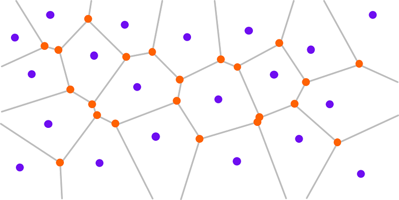
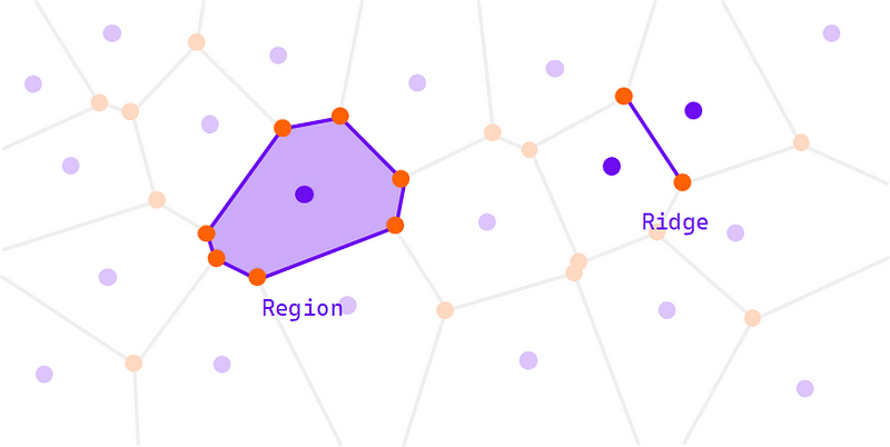
Voronoi diagram calculated using scipy.spatial. Image by Author.

scipy.spatial ‘s Voronoi returns a list of vertices, regions, and ridges, which are going to be useful later on.

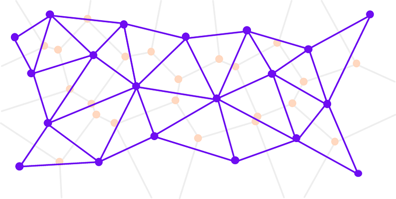
A region and a ridge in a Voronoi diagram. Image by Author.

These additional points help form what is called the Delaunay tessellation.

Delaunay tessellation on top of the Voronoi tesselation. Image by Author.

Lloyd’s Relaxation Algorithm

Now, we have to generate random points where cells will be.

If we use a function like random from numpy.random to generate multiple points and calculate its Voronoi diagram, we get these results:

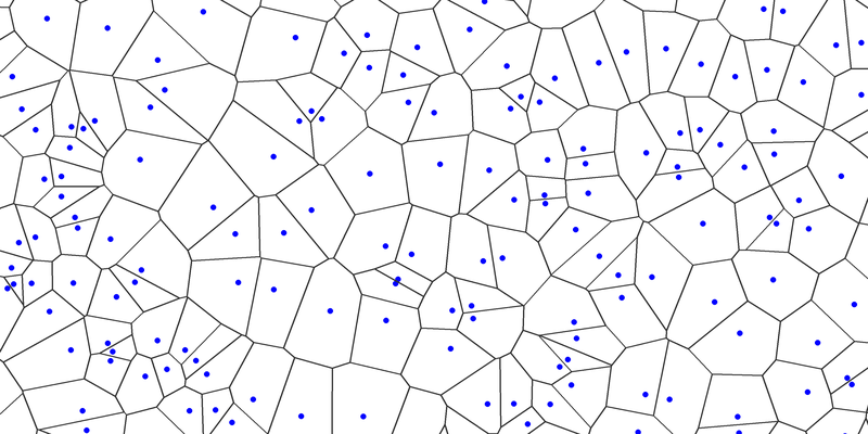
Voronoi diagram of random points. Image by Author.

You may have noticed that some points are too close to each other. This is known as clustering. Cells are supposed to be distributed uniformly.

This is more noticeable when we zoom out (or increase the number of points):

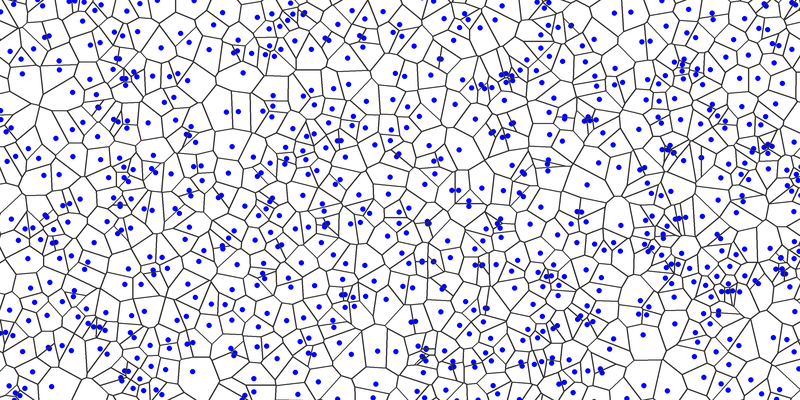
Notice how some points are clustered together while other areas are empty. Image by Author.

To solve this problem, we have to space the points apart.

One way to solve this problem is to use Lloyd’s relaxation algorithm, which takes advantage of the Voronoi diagram of the points.

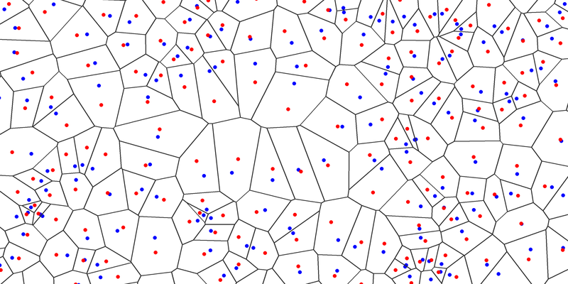
The idea behind Lloyd’s algorithm is to calculate the Voronoi diagram of our points, then move every point to the centroid of its cell. And repeat the process a certain number of times

The centroid of a polygon is the average of its vertices.

This is a Voronoi diagram with cell points in blue and cell centroids in red.

Voronoi diagram with cell points (blue) and cell centroids (red). Image by Author.

We can then, replace cell points (blue) with cell centroids (red) over and over again.

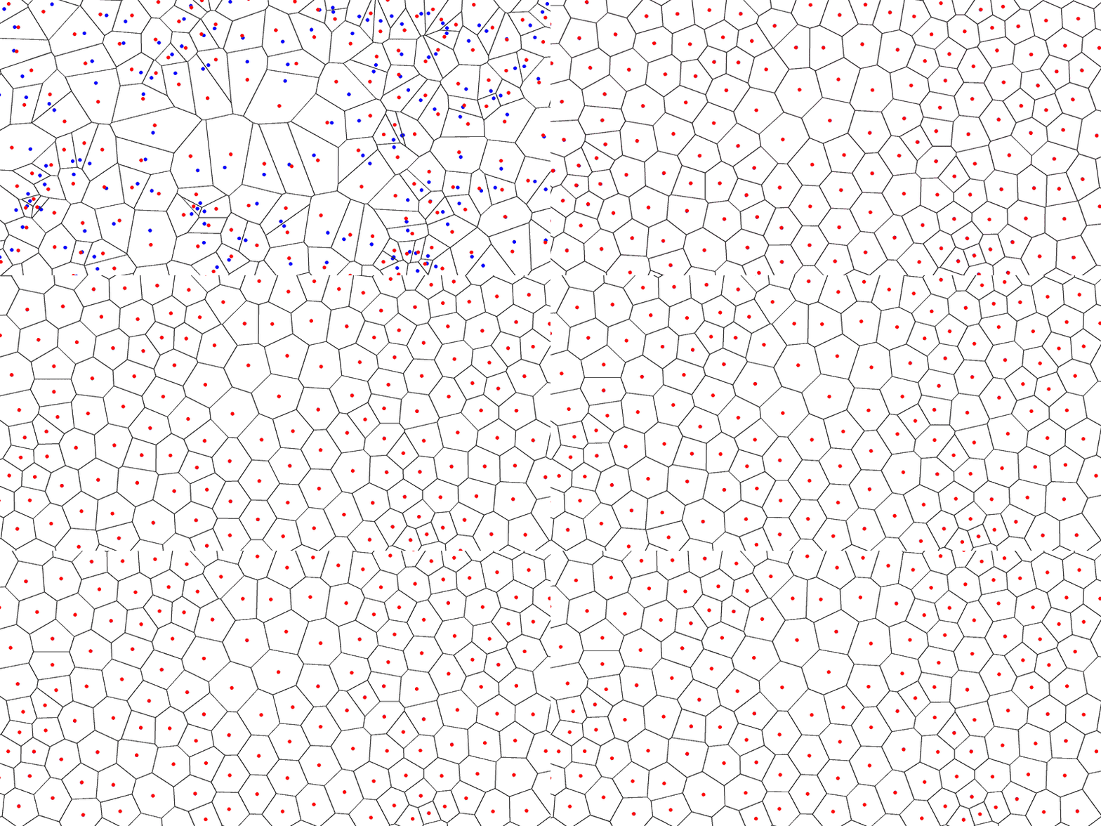
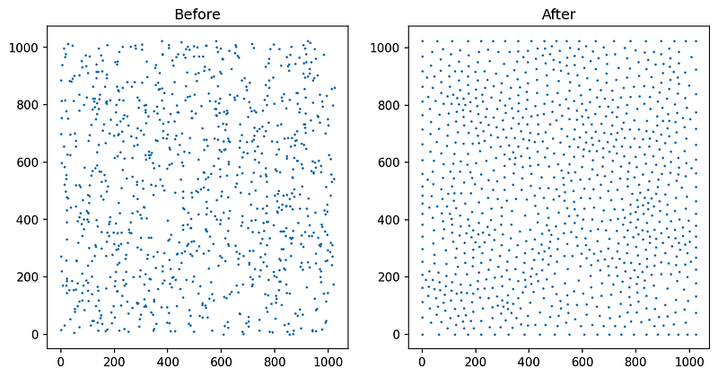
Lloyd’s relaxation algorithm animation. Image by Author.

This yields better looking random points.

Perlin/Simplex Noise: Why do we need it?

In order to generate random terrain, we have to generate properties that vary randomly through space, properties like elevation, temperature, or precipitation.

One could think of using random , and that would make sense.

We are going to generate a random number, between 0 to 255, for every block on the xy-plane in our world.

This yields the following result:

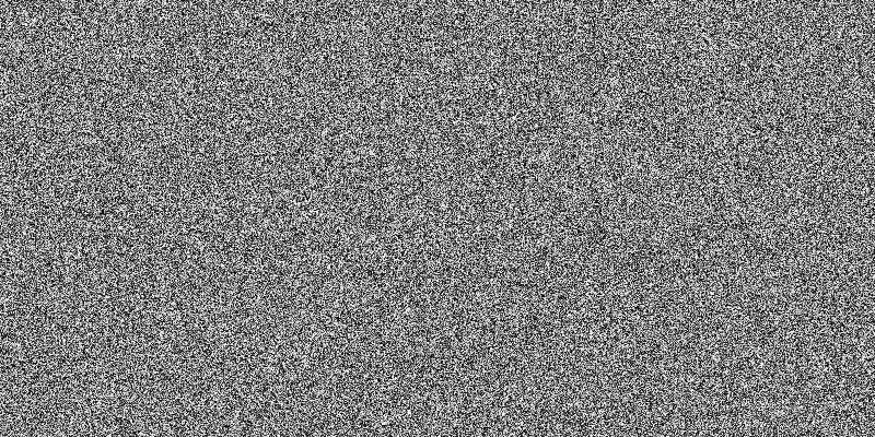
Well, that looks more like a QR code than a Minecraft world.

The problem is that our random values have no coherent structure. Every value is individually generated and has nothing to do with its neighboring ones.

To overcome this problem, we are going to use Perlin noise.

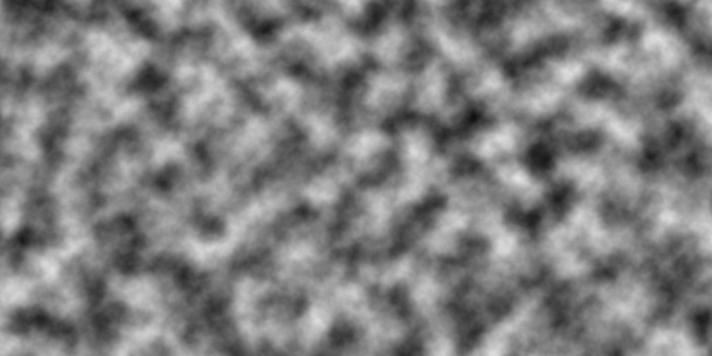
Perlin noise was invented by Ken Perlin in 1983. Unlike regular random noise, it has a structure to it. It looks closer to random patterns found in nature (clouds, forest distribution).

Simplex noise was also created by Ken Perlin himself. It has many advantages over Perlin noise. Perlin noise and Simplex noise are being used today in almost all of procedural generation.

We will use an implementation of Simplex noise in Python called noise. (Python module).

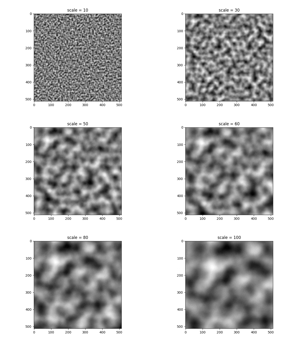
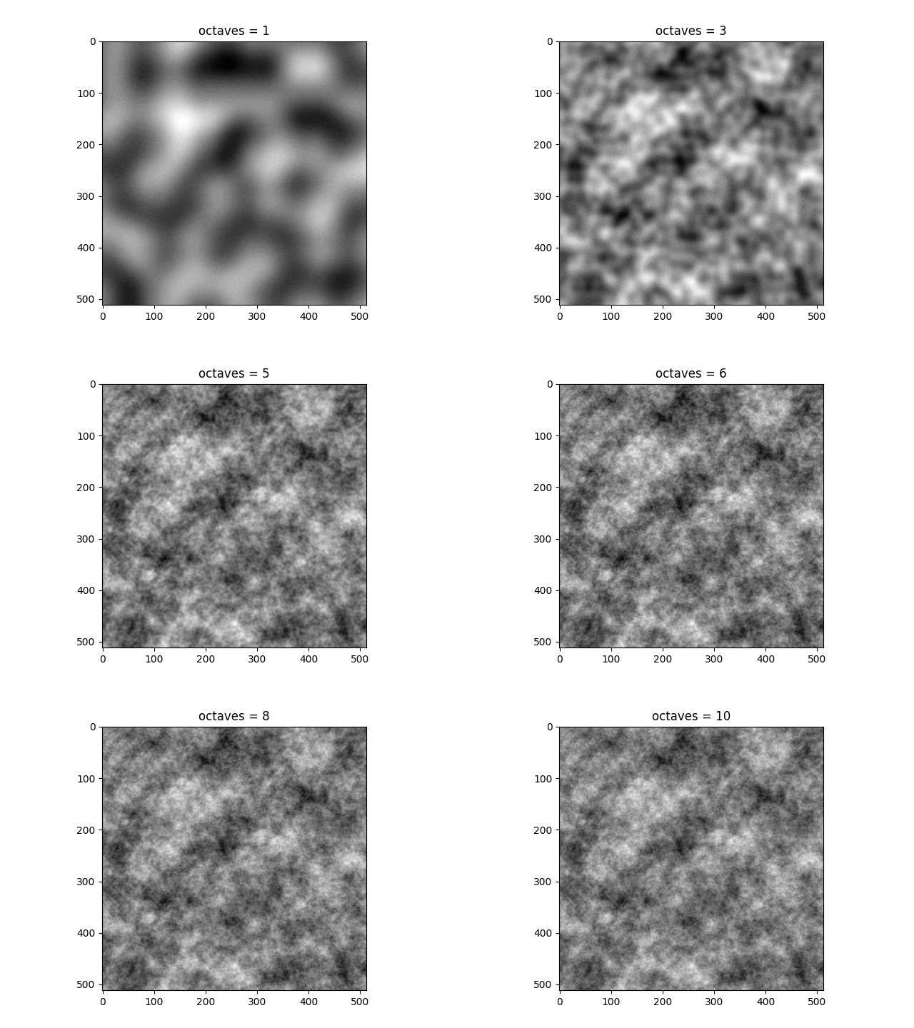
We have 4 variables to play with: scale, octaves, persistence, lacunarity. I won’t explain what each one does, but I will leave you with these GIFs I made to get a sense of it yourself.

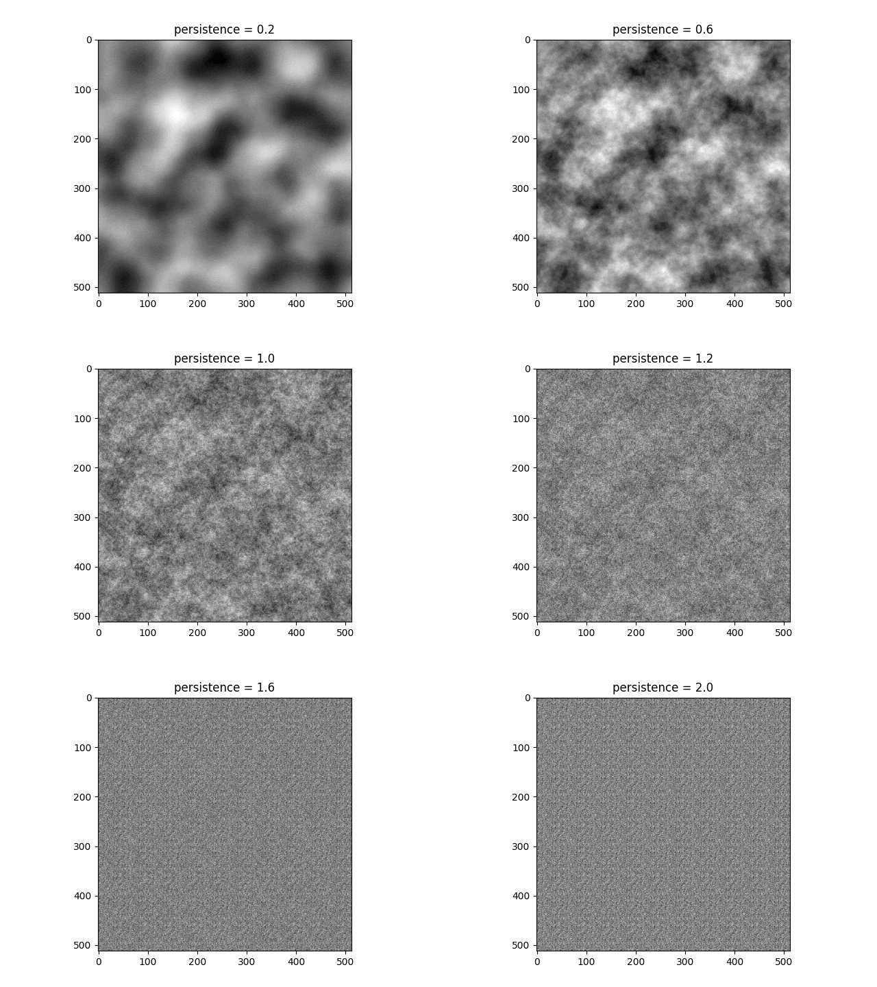
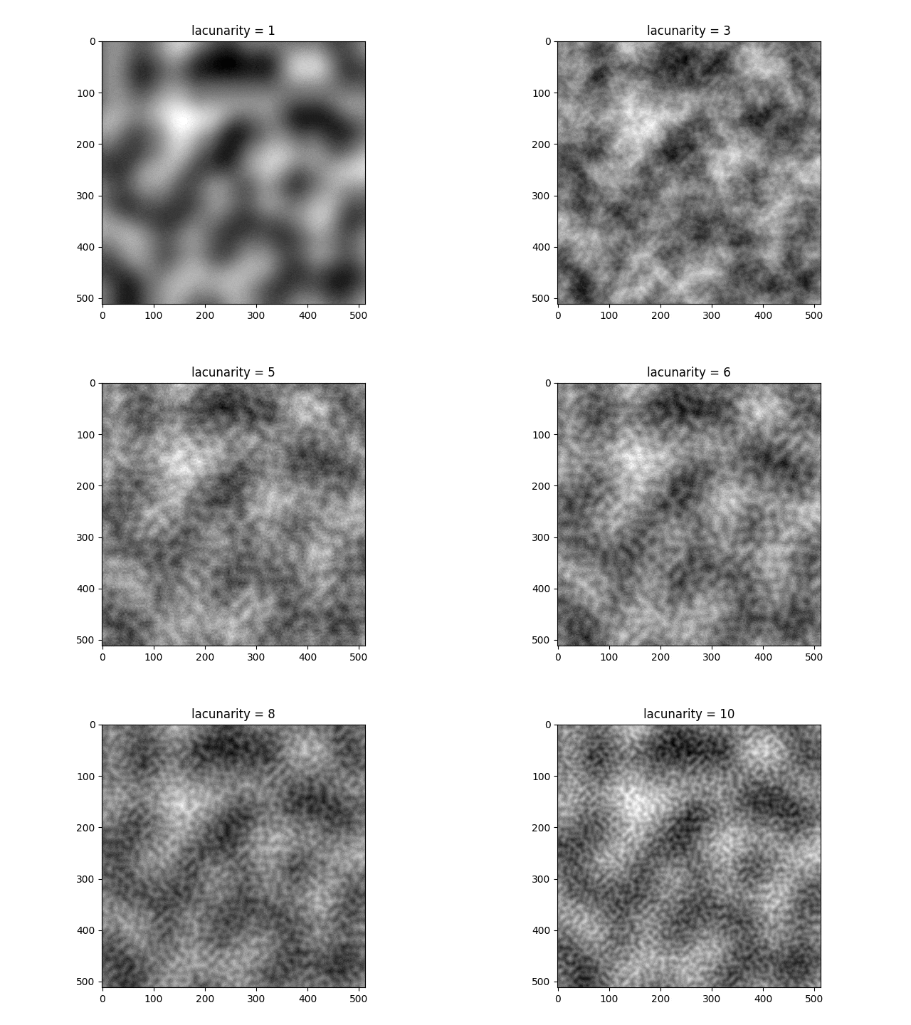
Perlin noise with changing parameters. Image by Author.

The returned noise values are between -1 and 1.

Regularity of cells — Blurring the boundaries

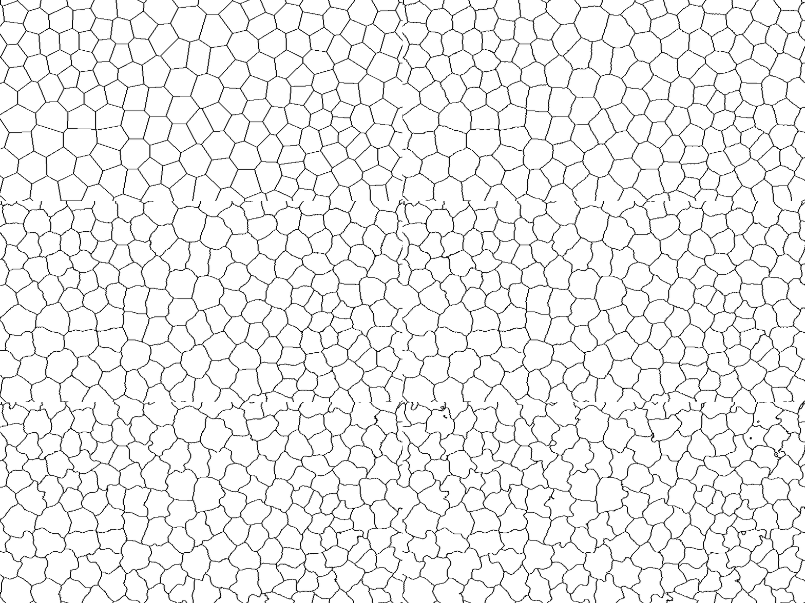
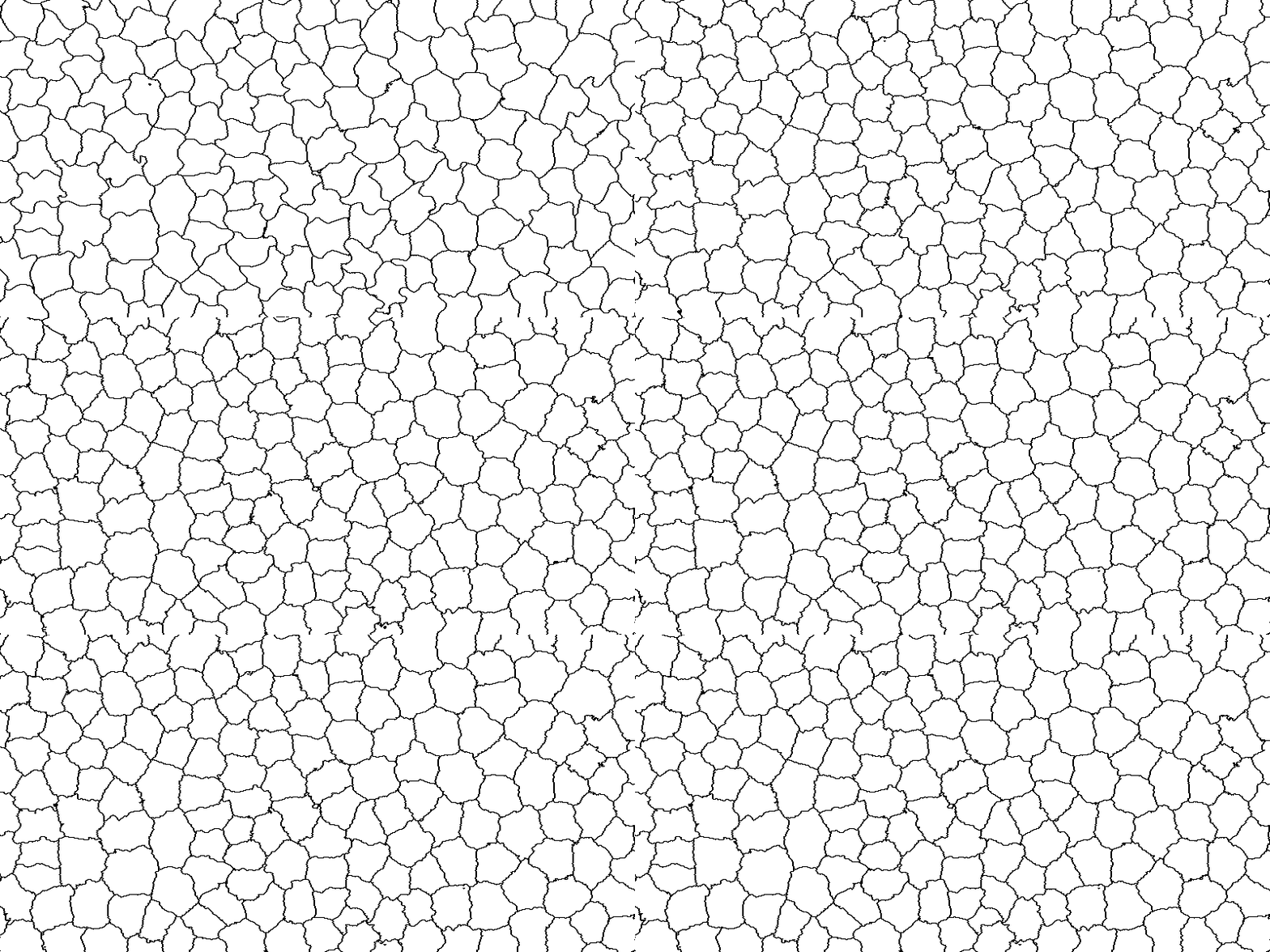
Although the points we generated above for the cells are nicely spaced apart, our cells look almost like regular polygons.

To overcome this problem, we will use Perlin noise. For every point, we will select a random point in its neighborhood and assign the newly selected point’s cell to the current point.

For this, we need two noise maps, one for the displacement in the x-axis and another for the y-axis.

We can control the noisiness of the boundaries by multiplying the noise (values between -1 and 1) by a constant length.

Boundary noise length animation. Image by Author.

Boundary noise octave animation. Image by Author.

Choosing Biomes

Minecraft has more than 60 different biomes. Each with different properties. Now that we have divided our world into cells, we have to assign a biome to every cell. We will use Perlin noise for this.

Temperature–Precipitation graph

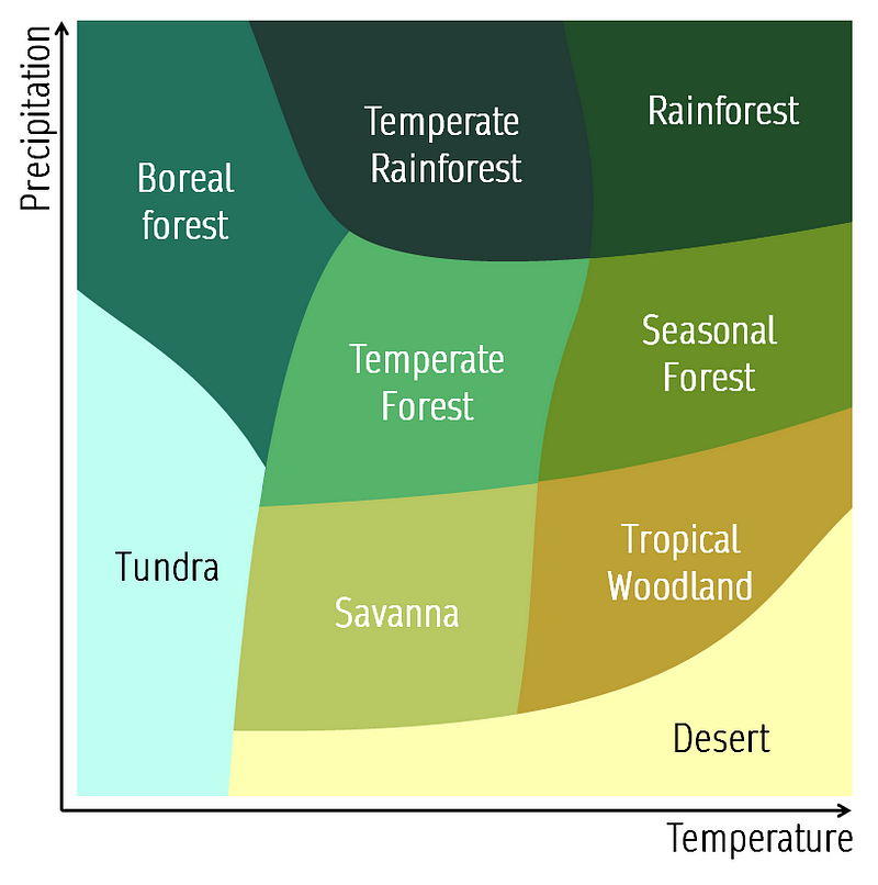
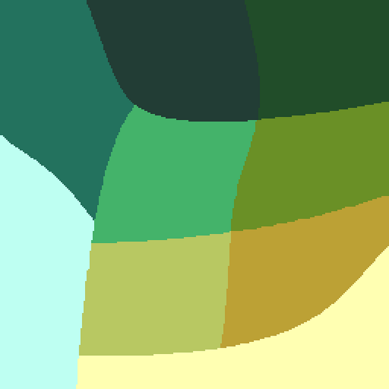
We will define biomes based on two parameters: temperature and precipitation, using a temperature–precipitation graph. This is how biomes are usually defined in environmental biology.

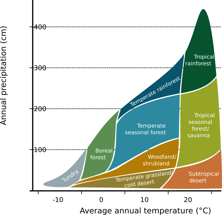
*“Climate influence on terrestrial biome” by Navarras is in the Public Domain, CC0*

We will use this graph as an inspiration to design our own temperature–precipitation graph.

Temperature–precipitation graph. Image by Author.

Temperature and Precipitation Maps

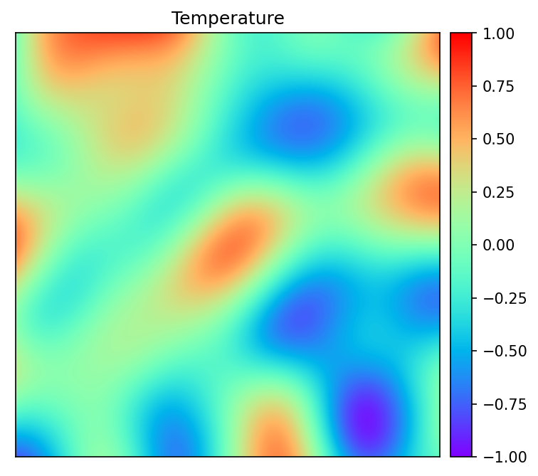
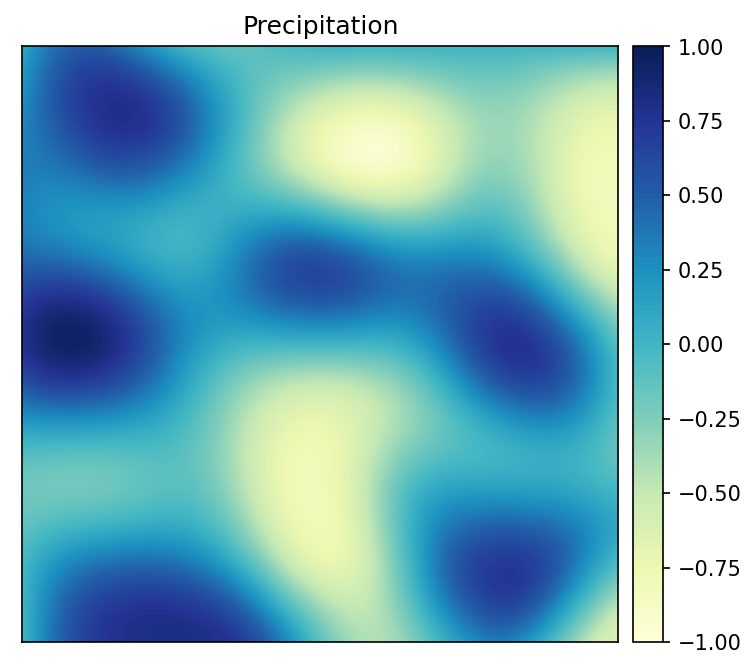
Now, we will assign to every cell a temperature and a precipitation value using Perlin noise. We will generate two maps each containing noise values for all blocks in our chunk.

Temperature and precipitation maps. Image by Author.

Histogram Equalization

If we use the temperature and precipitation maps above, we will encounter a problem. The Perlin-noise-based values are not uniform. There are more values close to 0 than values close to -1 or 1. This discriminates biomes that are on the edges of the temperature–precipitation graph.

To further understand this non-uniformity, I plotted 1D-histograms and an amazing-looking 2D-histogram of the temperature and precipitation maps.

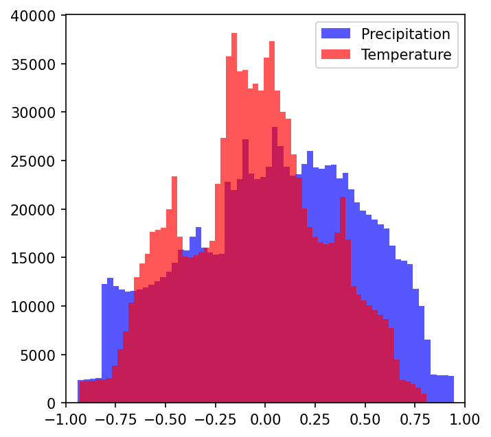
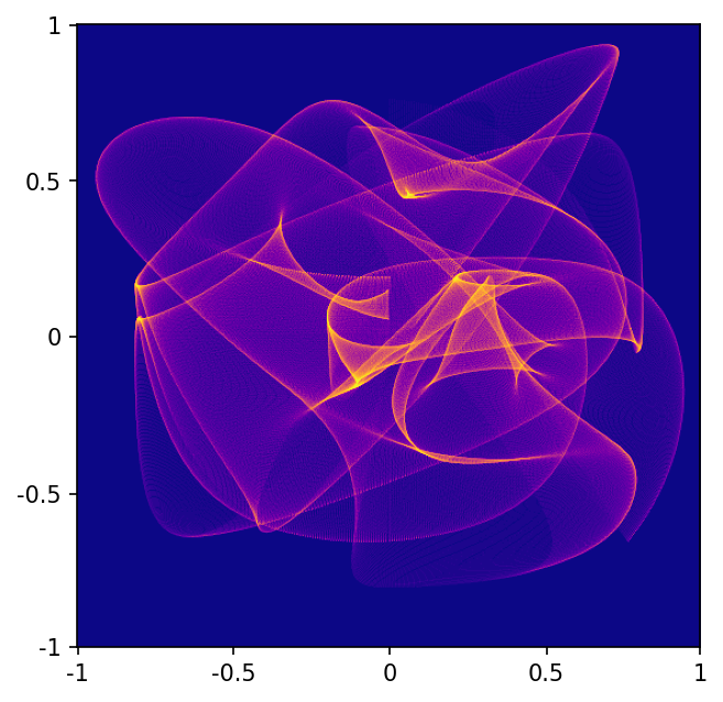
1D histogram (left) and 2D histogram (right) of the temperature and precipitation maps. Image by Author.

As you can see, values at the edges are discriminated against. To solve this, we will equalize our values.

Histogram equalization is used to adjust the exposure of an image. For this reason, I used skimage‘s exposure function.

An equalized histogram is flat.

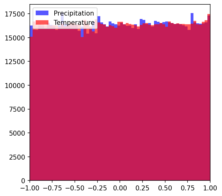
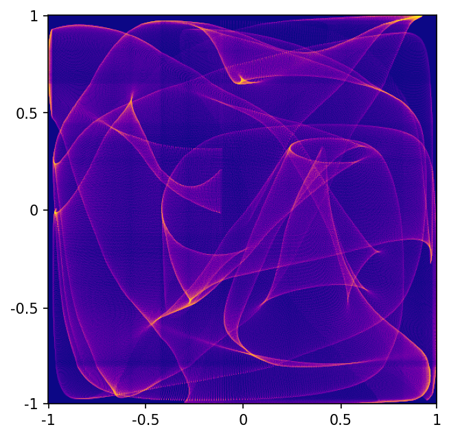
Equalized 1D histogram (left) and equalized 2D histogram (right) of the temperature and precipitation maps. Image by Author.

Since we equalized temperature and precipitation separately, the 2D histogram is not fully flat.

We might not want our histograms to be fully flat. If we want to have some control over the flatness of the histograms we can blend the unequalized values the equalized values.

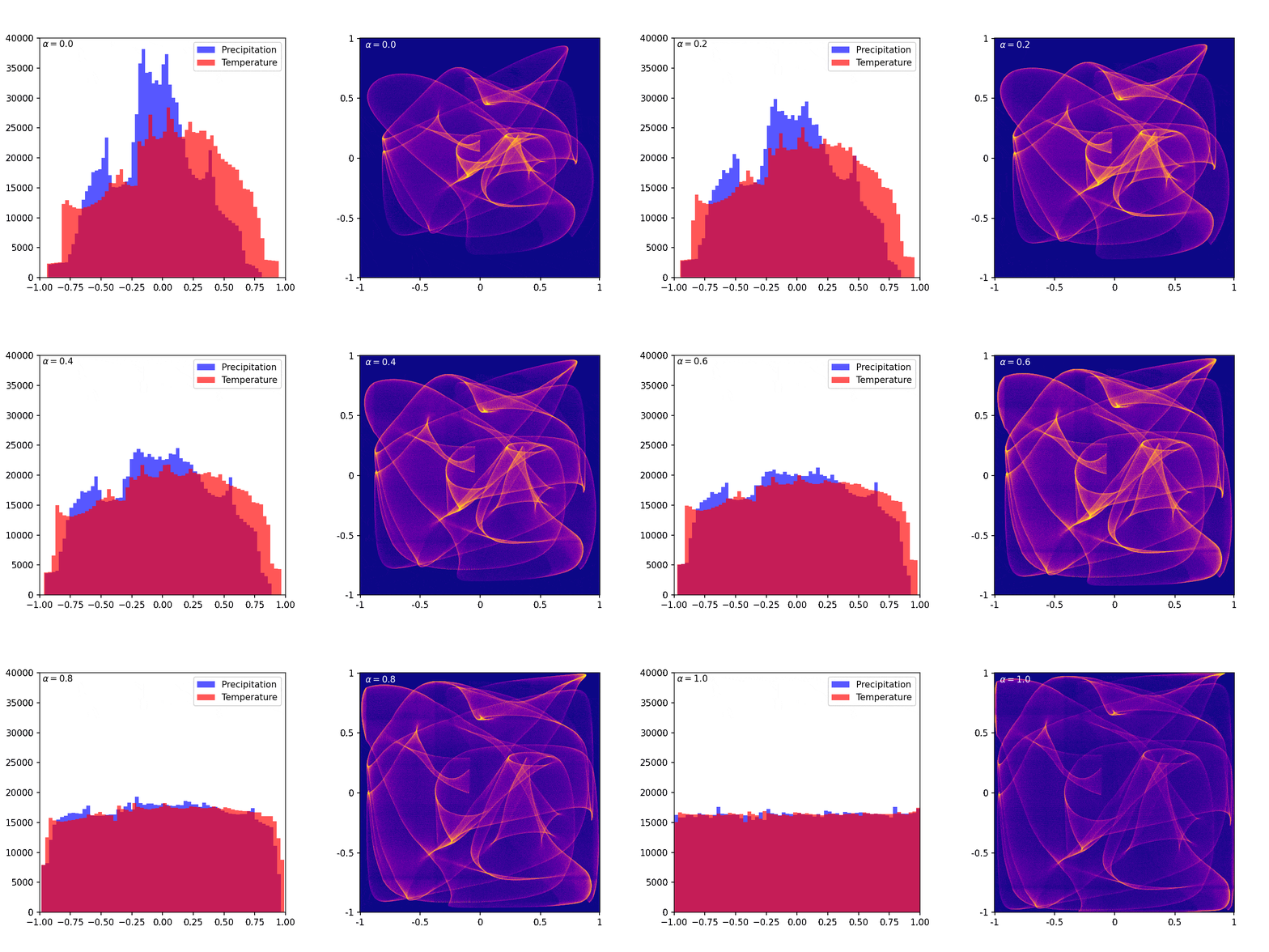
Animation of histogram equalization. Image by Author.

Now, we can control how equalized our values are.

Averaging Cells

We will average the maps inside every cell to get the temperature and precipitation values for every cell.

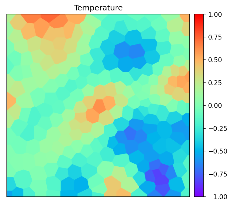
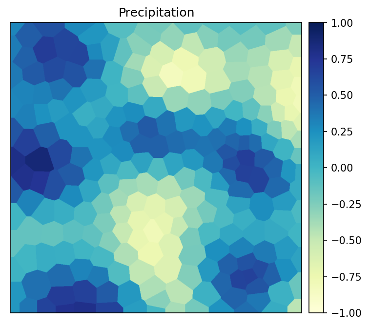
Cellular temperature and precipitation maps. Image by Author.

Now, every cell has a temperature and a precipitation value between -1 and 1.

Quantization

To simplify the way we work with temperature and precipitation values, we will convert them into integers. We will use np.uint8 as a data type to store these values.

To convert the values in the maps above, we will map them to [0, 255] and round the value to the nearest integer.

Quantization doesn’t change how the temperature and precipitation look.

We can, now, define our temperature–precipitation graph by a 256×256 image.

Biomes Map

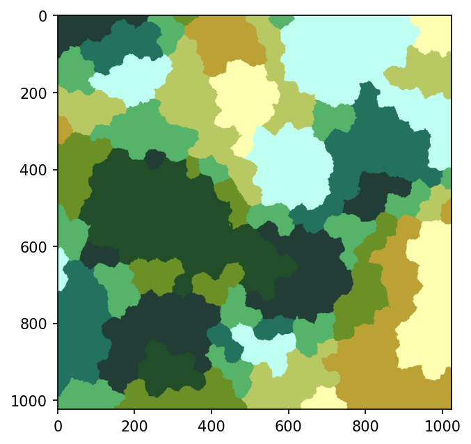
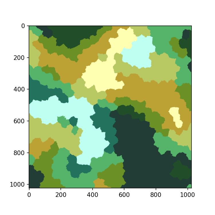
We can assign to every cell a biome using the temperature–precipitation graph, temperature map, and precipitation map. Doing this for every cell yield these results:

Height Map

Every point in our 2-dimensional world has an elevation (height). To generate a height map, we will use a noise map.

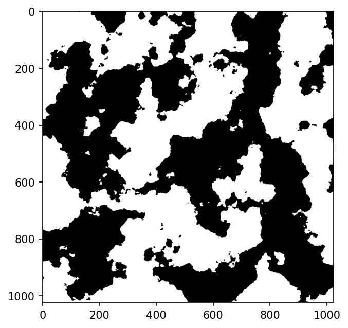
Using this height map (with values between -1 and 1), we can create a lank mask. Values above 0 are land and values below 0 are sea.

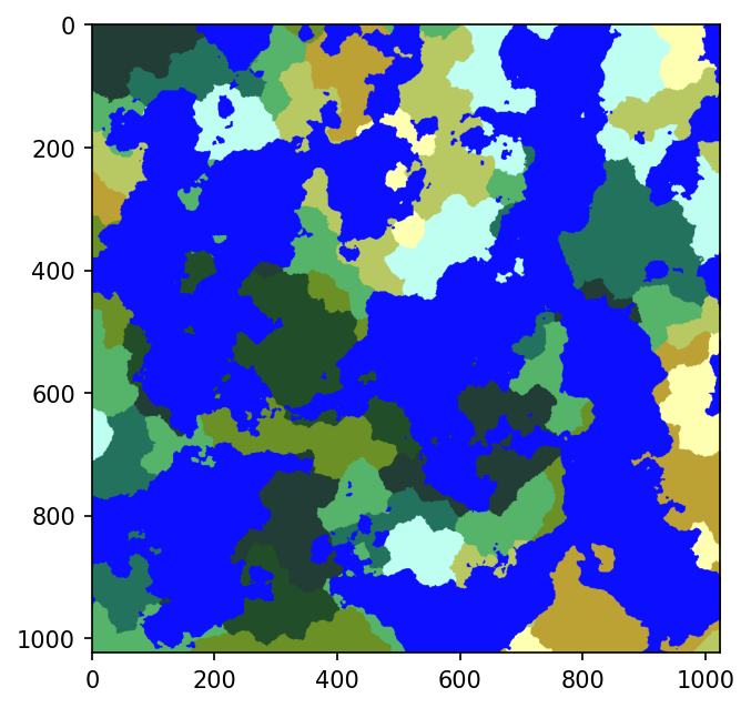
Combining this with the image generated before:

Biome map with land mask applied. Image by Author.

To visualize the height, we will add some shading to the map.

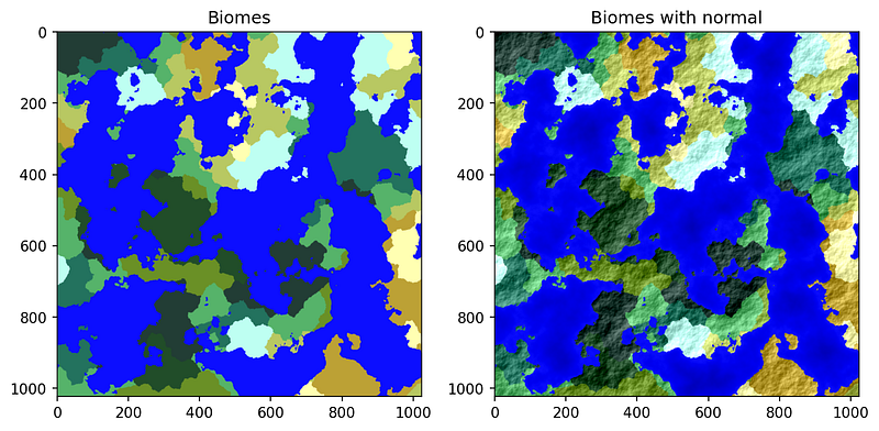
Biome map with land mask (left), shaded biome map with land mask (right). Image by Author.

So far, the results look promising. But the height is independent of the biome. We need to change the height map within each biome. We will achieve this by applying a function on the height map.

Height Map Detail

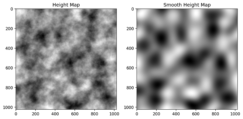
We will use 2 height maps with different levels of detail. This is done by changing the number of octaves in the Perlin noise.

Here are our 2 height maps:

Sharp (left) and smooth (right) height maps. Image by Author.

Height Map Filters

We will work with the height map in land (values between 0 and 1). Every biome will use a combination of the two height maps (smooth and sharp height maps). And then apply a filter (function) to it.

The idea of applying filters is going to be inspired by Photoshop’s curves. We will use Cubic Bézier Curves to define a function which we will apply to the height map.

Here are some examples of filters:

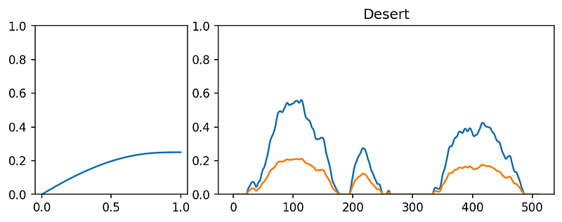
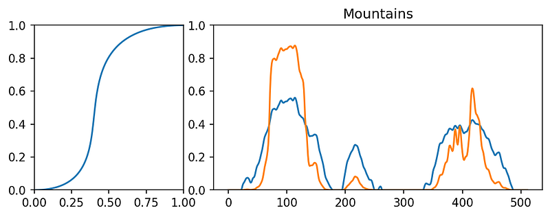
We will create and adjust a filter for every biome.

Desert, savanna, and tropical woodland filters. Image by Author.

Tundra, seasonal forest, and rainforest filters. Image by Author.

Temperate forest, temperate rainforest, and boreal filters. Image by Author.

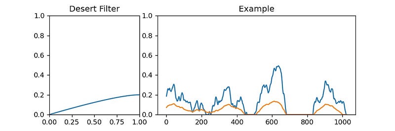
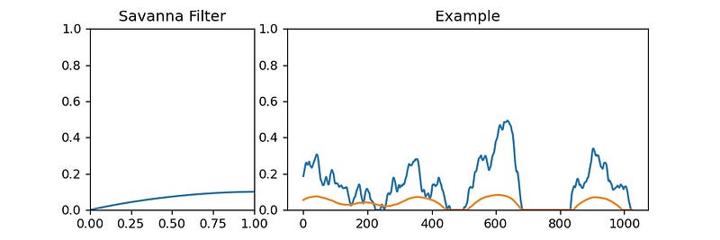
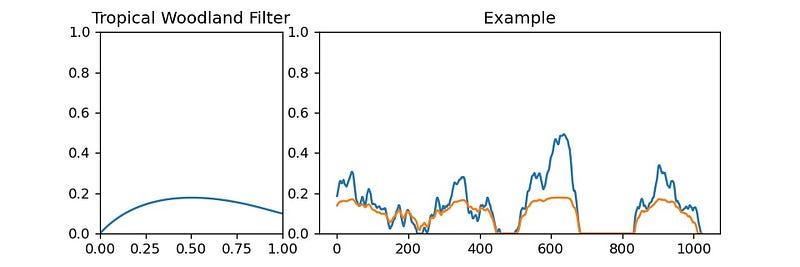
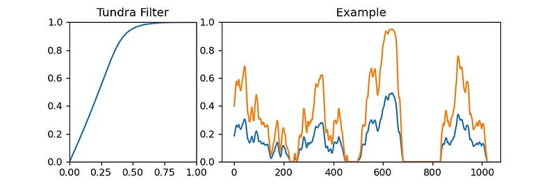
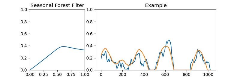
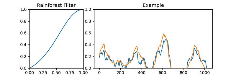
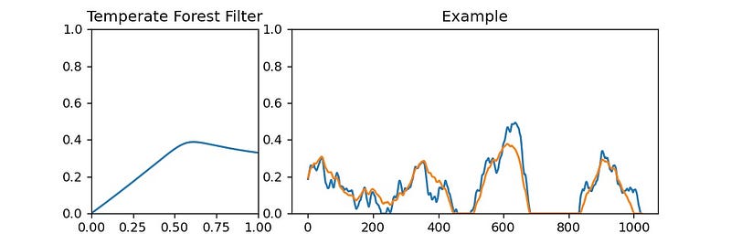
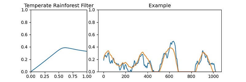
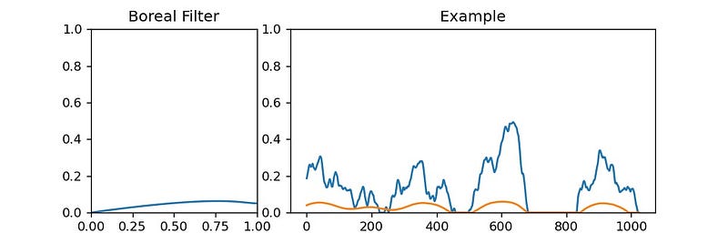
To apply these filters to our height map, we will use masks. A mask is a map containing 1 in areas of a certain biome and 0 in the other areas.

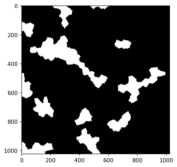
If we use a hard map, we will have huge height variations. That is why we will feather the masks before using them. And we will also remove the ocean from this map (by multiplying it with the land mask), so we only apply the filters to land.

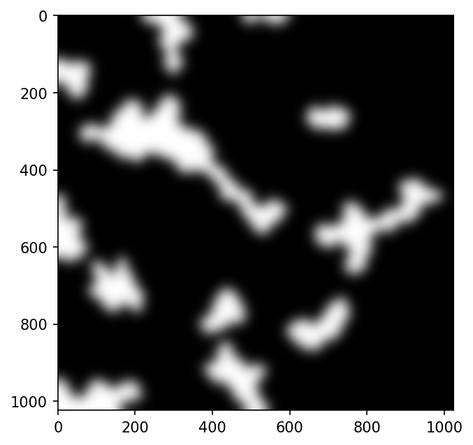
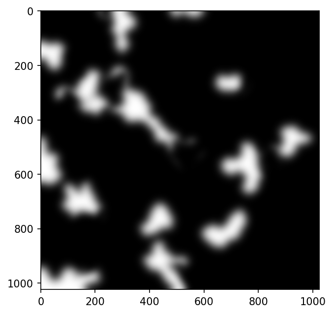
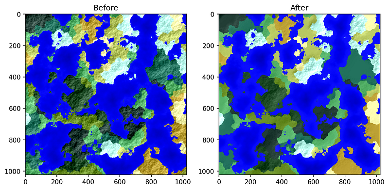
A feathered (blurred) biome mask (left), only land (right). Image by Author.

We will apply the filters of every biome on the height map using the masks above. We get the following results:

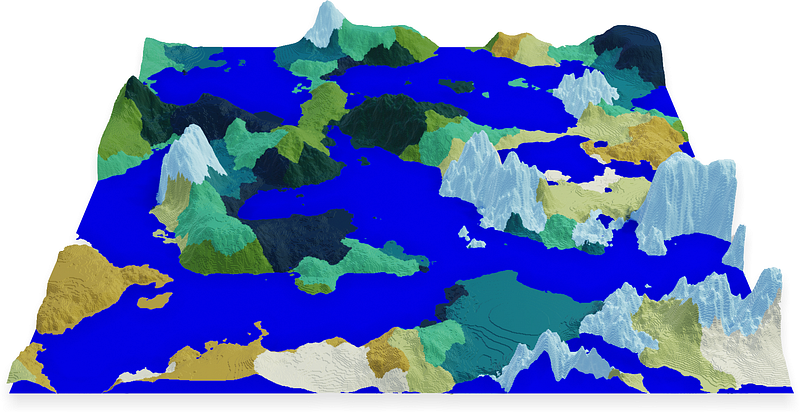
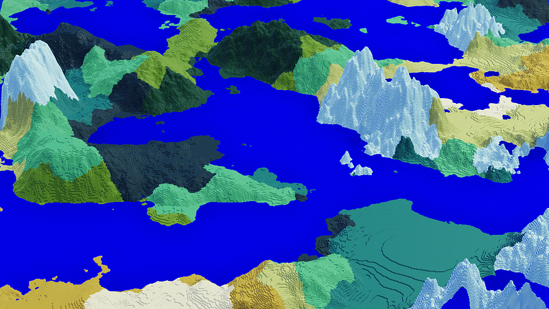
Final Height Map Results in 3D

We can use Blender to render these maps in 3D. We’ll use the height map in the displace modifier in Blender.

Render of height map with colored biomes. Made using Blender. Image by Author.

Rivers and lakes

Boundaries

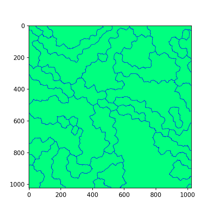
We will add rivers between the boundaries of biomes. First, we need to calculate the boundaries between the biomes.

To do this, we will loop through every point on the map. If the point has all its neighbors of the same biome then it is not on the boundary. If it has more than one type of biome in its neighbors, then it is part of the boundary.

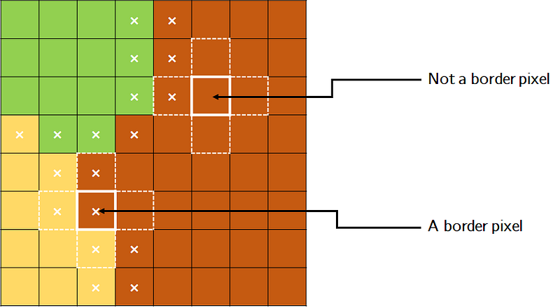
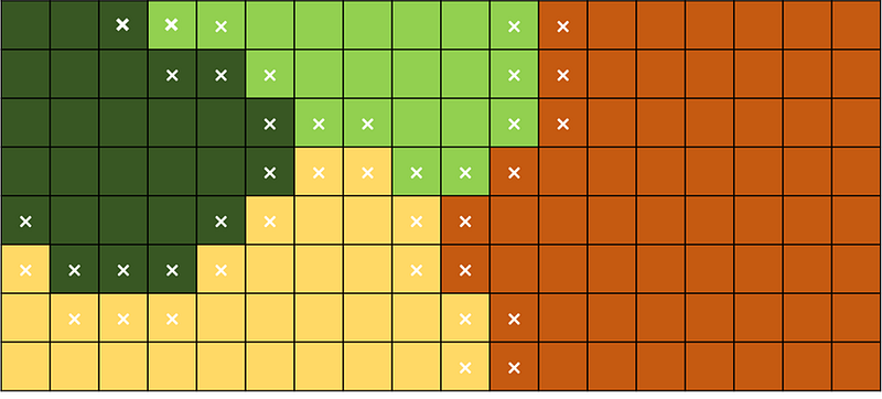
Illustration of a border pixel. Image by Author.

Applying this technique to our biome map yields the following results.

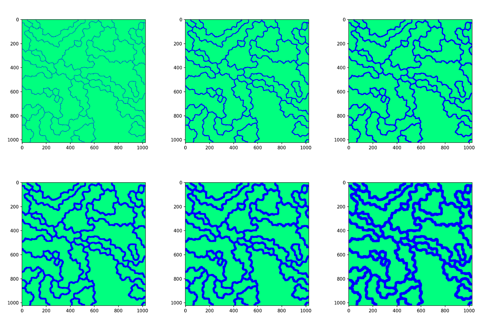
Biome map (left) and rivers (right). Image by Author.

We can control the size of the rivers by changing the size of the box that contains the neighbors.

Rivers with varying sizes. Image by Author.

We will use 2 different kinds of rivers: biome rivers and cell rivers. Biome rivers are big and placed on the boundary of biomes, while cell rivers are smaller and placed on the boundaries of cells. We then use the land mask to limit rivers to land.

Rivers will also be limited to medium and low altitudes.

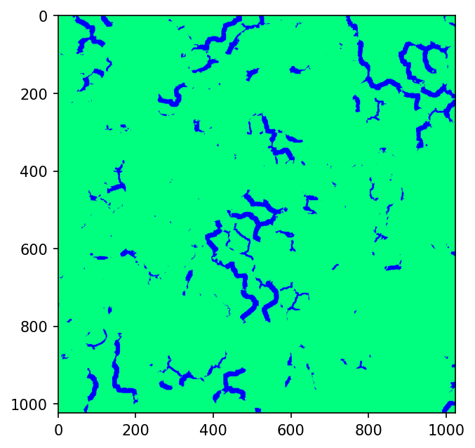
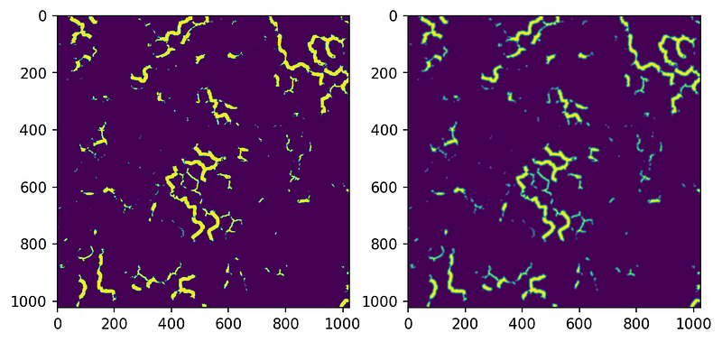
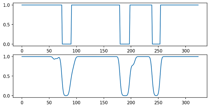
We will use this river mask to change the height map. We will blur this river mask and then use the original river mask to mask it. This creates a map with high values in the middle of the rivers that slowly fade to low values at the edges of rivers.

Here is a comparison of the river mask with the blurred and masked river mask.

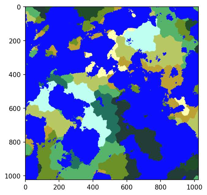
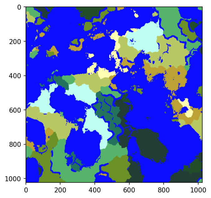
Cross-section of the river mask. Image by Author.

We will use this map to “carve” rivers in the height map.

Biome map (left) and biome map with rivers (right). Image by Author.

Trees and Vegetation

To add trees to our map, we will use Lloyd's Relaxation Algorithm discussed previously. This sampling method helps us generate random points that are spaced apart.

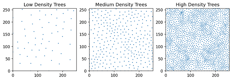
Randomly sampled points (left), Relaxed points (right). Image by Author.

We will generate sets of trees with different densities depending on the biome.

Varying levels of tree density. Image by Author,

We will combine a set of trees with the biome masks and land mask discussed before to fill biomes with trees. Every biome has a different density and, of course, different types of trees.

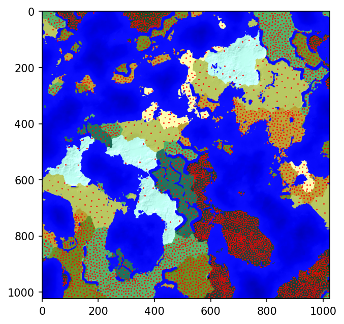
My Blender skills restrain me from visualizing the map in 3D with the trees :(.

Source Code

Here is a Jupyter notebook containing all the steps in the article in code.

Warning: The code is very messy and undocumented.

Conclusion

Procedural generation is a very powerful part of computer graphics. It makes generated content feel random yet artistic and structured. As said before, this can be used in machine learning to generate datasets that cover areas that are hard or expensive to cover using normal real-world data gathering.

This article was just a fun project that I wanted to work on for more than a year. I learned many concepts along the way and I had a lot of fun. It is still lacking a lot. For example, I need to create caves underground, villages, and create an algorithm that can combine chunks seamlessly.

Inspiration

I got inspired by many articles when writing mine. If you enjoyed this article, then you’ll definitely want to read these, too:

You can also check out my previous article on Traffic simulation in Python, which covers how to procedurally generate traffic data.