Reinforcement Learning: SARSA and Q-Learning — Part 3

Introducing the Temporal Difference family of iterative techniques to solve the Markov Decision Process

In the previous article — Part 2 — we discovered a few solution algorithms to solve the Markov Decision Process (MDP), namely the Dynamic Programming method and the Monte Carlo method. The Dynamic Programming approach can be easily applied when we know the entire environmental dynamics of the MDP, such as the Transitional Probabilities between all states (conditioned on actions). However, such assumptions may not be practical, especially when we consider real-world applications, when stochastic relationships between states and actions are often vague.

Without knowledge of Transitional Probabilities, we then introduced the experiential learning with the idea called Monte Carlo learning. Under this paradigm, there is a learning agent navigating its environment with actions taken from an updated “best-guess” policy after every episode. Under trial-and-error with this paradigm, the policy then updates itself only after every episode.

To refresh or revisit these ideas, check out Part 2 below:

However, as mentioned in the preceding article, the above solutions are limited in applications — especially in Model-free scenarios when you need to update your policy on the go before the episode ends. Or perhaps the episode is never-ending — imagine framing life’s journey as an MDP. In this case, we are usually updating our learning — what best actions to take — continuously, rather than waiting until a certain juncture or even until the end of our lives.

To solve this case of learning continuously across time steps, this article will explore the Temporal Difference (TD) family of algorithms, namely SARSA(0), SARSA(λ), and Q-Learning. Both SARSA(0) and SARSA(λ) are On-Policy variants of Temporal Difference learning, while Q-learning is its Off-Policy variant.

1. Introduction to Temporal Difference Learning

Before we formally introduce SARSA(0), we will introduce the mathematics for Temporal Difference algorithms, which follow a similar intuition. To begin, let us first revisit the mathematics of Monte Carlo:

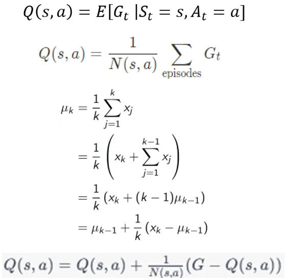
Recall that in each incremental update of Q(s,a) , the equation uses a sample of the Return G , which requires a complete episode. However, in the Temporal Difference algorithms, instead of sampling, we estimate the Return G , with the Bellman Equation, based on a one-step look ahead.

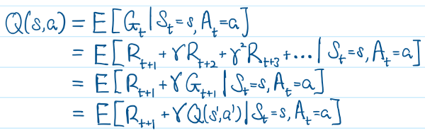
From the above, we are estimating the Return G with the iterative expression R + γ*Q(s',a') from the Bellman Equation. Hence, the incremental update becomes:

Note that when we initialize the MDP, all Q(s,a) are arbitrary (guesses), hence in every iteration R + γ*Q(s',a') is only an estimate. Thus, in the incremental update above, we have approximated the 1/N(s,a) factor (in the Monte Carlo case) with the constant α factor.

Note: If we apply Monte Carlo learning to a non-stationary MDP, we should also approximate the 1/N(s,a) factor with α factor.

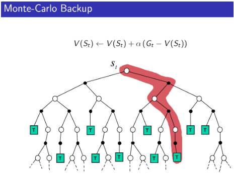
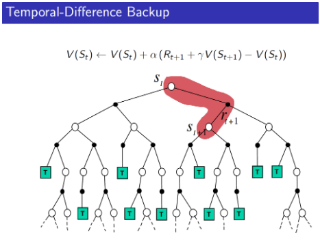
As you can see, both Temporal Difference and Monte Carlo use a similar incremental update algorithm. But there is a distinction. In Monte Carlo, this incremental update can only happen for all visited states after an entire episode, when you have sampled the Return G . On the other hand, in Temporal Difference once you have proceeded to the next time step t+1and obtained the Reward R_{t+1}in the process, you can immediately update the Q(s,a) for the single, visited state in the preceding time step. Hence, for Temporal Difference learning, updating of Q(s,a) values takes place continuously (for visited states) before an episode ends.

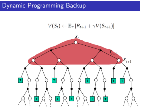
In addition, if you have followed the previous article in Part 2, you would also have noticed some similarities between the Dynamic Programming and Temporal Difference algorithm. Both applied the Bellman Equation iteratively in a single-step bootstrapping fashion — that is you begin the algorithm with a randomly initiated estimate of the Q(s,a) or V(s) . With each iteration, the value functions become an increasingly more accurate estimate. As explained in Part 2, this is because you are adding the true Reward R_{t+1} to the estimate at every iteration, allowing the estimate to gradually converge to the true value function.

With these in mind, we will illustrate these distinctions among Temporal Difference, Monte Carlo, and Dynamic Programming below in the context of the State-Value Function V(s) :

2. SARSA(0) — The Single State Backup

Moving on, we are ready to formalize the SARSA(0) algorithm. The SARSA(0) algorithm is basically the vanilla Temporal Difference (TD) algorithm and the preceding section has already covered most of its ideas. You may also ask why we call it ‘SARSA’ — the diagram below illustrates the idea:

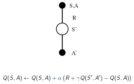
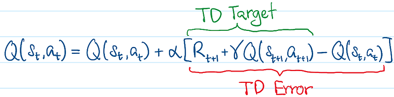
‘SARSA’ basically means the incremental update in each iteration occurs across a single time step — State-Action-Rewards-State-Action. Here, we will also introduce additional vocabulary for the SARSA incremental update — the TD Target and TD Error:

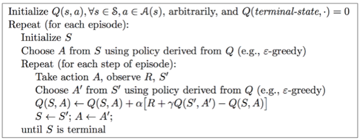
Now, the SARSA(0) algorithm executes the Temporal Difference paradigm in its raw form. That means, for a particular trajectory, at every time step, only Q(s,a) in the immediate, preceding time step is being updated — there is only a one-step look ahead.

This means when you arrive at a new state and took a certain action, then retrospectively, you realize how good or bad the immediate preceding state-action pair was. However, the downside is that you cannot retrospect on state-action pairs that occurred a few time steps ago. We illustrate the SARSA(0) algorithm below:

3. SARSA( λ ) — The Multi-State Backup

If we want to update the Q(s,a) for all visited states in all preceding time steps, based on the Rewards and Q(s',a') at the latest time step, then SARSA(λ) is the solution. However not all visited state-action pairs are updated equally — the more recently visited state-action pairs, relative to the latest time step, have greater weightage in the Q(s,a) update. The SARSA(λ) algorithm uses the idea of Eligibility Traces to capture this idea:

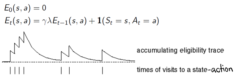
From the above illustration, the SARSA(λ) algorithm gives a new variable, E_{t}(s,a) , initialized to zero, to all possible state-action pairs. At every time step in the episode, if the state-action pair is visited, we add 1 to it. At the same time, regardless of whether the state-action pair was visited, the eligibility trace E_{t}(s,a) is decayed by a factor of γλ , where γ is the discount factor and λ is the parameter of SARSA. Then for every state-action pair visited, we apply the incremental update as follows:

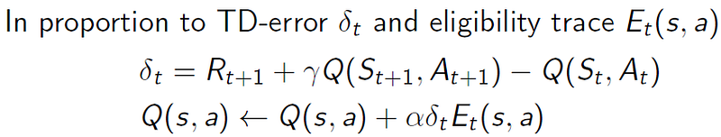
Of note, in each iteration (time step progression), the latest TD Error from the latest visited state is still computed based on a one-step look ahead, and the Q(s,a) for all visited states is updated simultaneously with that most recent TD Error, together with their Eligibility Traces. Hence at every iteration, the Q(s',a') and rewards R from the most recent time step will propagate, in proportion, to the earlier visited states. We formally illustrate the SARSA(λ) algorithm below:

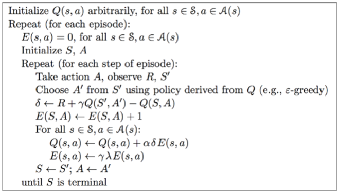
Also note that, similar to SARSA(0) and also Monte Carlo, at every iteration, the SARSA(λ) follows the Policy Evaluation and Policy Improvement paradigm, as it is doing On-Policy learning. The eligibility trace variable is also reset to zero at every new episode.

In hindsight, the SARSA(λ) algorithm is powerful because it allows the learning to be truly online. Recall the car driving example in the conclusion section in Part 2, where we talked about a near car crash during the mid-journey. Perhaps the car crash nearly occurred because of some poorly judged actions that occurred a few states before, rather than the actions in the immediate preceding state. Using SARSA(λ), the Q(s,a) of the series of preceding states can be immediately updated, at the state where the near car crash occurred. Therefore, in the later part of the journey, if the driver were to revisit these states, or states similar to these, he would be able to take early pre-emptive actions to prevent another possible car crash from occurring several states later.

Note: Based on the above formulation, the SARSA(λ) becomes exactly the SARSA(0) paradigm, when we set λ=0.

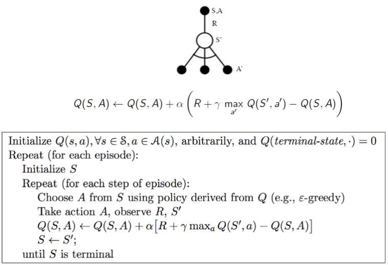
4. Q-Learning — Off-Policy TD Algorithm

Moving on, Q-Learning is an Off-Policy learning algorithm compared to SARSA(0)and SARSA(λ), which are On-Policy. If you need to refresh on the distinction between On-Policy and Off-Policy, do remember to check out the previous article in Part 2.

Q-Learning is more analogous to SARSA(0) than SARSA(λ), because both Q-Learning and SARSA(0) are one-step methods. Q-Learning does not utilize eligibility traces to spread learning updates backward through time or state-action space. But let us take a look at the incremental update where Q-Learning and SARSA(0) differ:

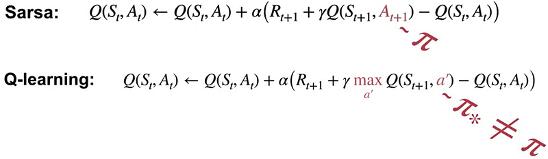
In SARSA(0), actions a are carried out with the exact same policy π that was learnt in the previous iteration. In Q-Learning however, the Behavior Policy (policy that carries out actions) follows the ϵ-greedy policy w.r.t Q(s,a) while the Target Policy (learnt policy) follows the greedy policy w.r.t Q(s,a) . Although the Q-learning does not make use of Importance Sampling algorithm, as we have seen for Off-Policy Monte Carlo in Part 2, the difference in Target Policy and Behavior Policy makes Q-Learning truly Off-Policy.

Notably, in Q-Learning, while the choice of state and action is decided and selected by the ϵ-greedy policy w.r.t Q(s,a), the TD target in the incremental update of Q(s,a) is based on the estimated optimalQ*(s',a') — that is maximum Q value for state s’ — rather than the actual Q(s',a') that occurred. Depending on MDP, sometimes this property allows the Q-Learning to converge to the actual optimalQ*(s,a) faster than SARSA(0). And because we are learning optimalQ*(s,a) directly, this is why it is called “Q-Learning”.

We can think of Q-Learning this way: when we are observing someone performing a task repeatedly, at every action he performs, we can learn by forming a critical opinion of what alternative best action that he can take.

Below, we formally illustrate the Q-Learning algorithm:

5. Conclusion

Congratulations on reaching here — we have successfully explored the main variants of the Temporal Difference algorithms, which are important when we are considering Online Learning. Nonetheless, till now, we have only considered small discrete state-action space. If the state-action space is continuous in nature or extremely large, then it would be computationally infeasible to store every state-action values before retrieving them. For instance, if we were to consider real-world scenarios like training drones or robots to follow certain behaviors, then we have to frame the MDP like a continuous state-action space. How can we do so?

In the next article — Part 4 — we will begin to explore methods involving Function Approximation and apply deep learning techniques to solve for the optimal actions with particular continuous state features. So stay tuned, and check out Part 4 here:

P.S: Some of the diagrams and equations used in this article are adapted from the free lecture slides by David Silver and also the lecture slides in the Reinforcement Learning Specialization in Coursera.

Thanks for reading! If you have enjoyed the content, pop by my other articles on Medium and follow me on LinkedIn.

Support me! — If you are not subscribed to Medium, and like my content, do consider supporting me by joining Medium via my referral link.