Reinforcement Learning: Dynamic Programming and Monte Carlo — Part 2

Introducing two simple iterative techniques to solve the Markov Decision Process

In the previous article — Part 1 — we have formulated the Markov Decision Process (MDP) as a paradigm to solve any Reinforcement Learning (RL) problem. However, the overarching framework discussed did not mention a systematic solution to the MDP. We have ruled out using linear techniques — like matrix inversion — and briefly raised the possibility of using iterative techniques to solve the MDP. To revisit the idea of MDP, check out the Part I below:

From this article onwards, relating to RL, we will be discussing iterative techniques and solutions to the MDP. Namely, in this article, we will introduce 2 main iterative methods to solve the MDP — Dynamic Programming and Monte Carlo Methods.

1. Dynamic Programming

We will first talk about Dynamic Programming. Dynamic Programming is an iterative solution technique that makes use of 2 properties of the problem structure:

• The sub-problem can recur many times
• Solutions at each recurrence can be cached and reused

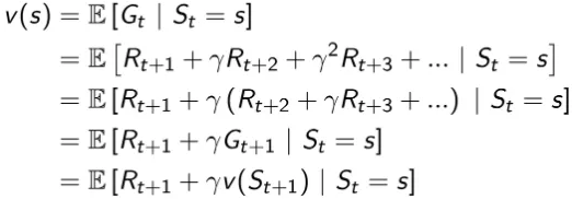
Hence, this is especially applicable to MDP problems, since the Bellman equation may give a recursive decomposition of the State-Value Function V(s) . Let us revisit the Bellman Equation for V(s):

However, the difference in Dynamic Programming is that for a particular policy π , we are using the Bellman Equation to map the neighbouring V(s') from time-step t to the current state V(s) time-step t+1 . The diagram below gives a similar intuition (the k variable below is the iteration step). Also, note that the below iteration is applied at every state in the Dynamic Programming algorithm.

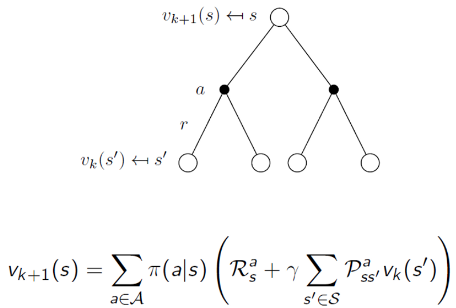
At this point, you may ask how would this work, especially when we do not even know the value of any V(s') at all. Nonetheless, we can begin the iteration by randomly initializing the values of V(s) every state. In fact, we even can set V(s)=0 for all states.

Here is the magic — after each iteration, the propagation of the true reward R(s,a,s') value adds to the inaccurate V(s) (which is also discounted) with the Bellman equation. Over many iterations, the V(s) becomes incrementally more accurate and converges to the true V(s) at every state for the MDP.

One important framework for Dynamic Programming in MDP is called the Policy Iteration, which we will explore next.

1.1 Policy Iteration

We should note that even Dynamic Programming for MDP is policy-dependent, if not who is to determine which next V(s') to consider? In the simplest case, we can take the uniform random policy to be fixed for every iteration. If we then evaluate based on this paradigm, the final value of V(s) every state can still be predicted at convergence. But this V(s) is only based on the naive fixed policy and not the true V(s) optimal policy, which we are interested in.

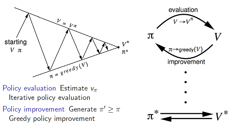
Now enter Policy Iteration, in which the Dynamic Programming is split into 2 steps — Policy Evaluation and Policy Improvement.

Again we can initialize the process with any policy and V(s) for all states. Typically we set the policy to be a uniform random policy — equal probability for each possible action in each state — and V(s)=0 for all states. In the first iteration, we start with Policy Evaluation, which is exactly the same process we described in the previous section. In the second half of the iteration, we apply greedy policy improvement: π'(s)= greedy(V(s')) . This new policy will then be applied in the succeeding iteration.

To illustrate, let us consider a simple MDP:

Consider a 4x4 Gridworld, and initiate initial V(s)=0 for all states with uniform random policy, where states (1,1) and (4,4) are terminal states. Rewards is -1 all every state except the terminal state (R=0). For simplicity allow γ=1, and let transition be deterministic.

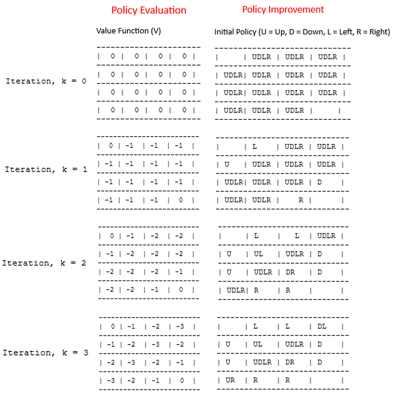
In the above simple example, the optimal policy has been achieved at the third iteration. In other more complex examples, the optimal policy may be achieved long before V(s) converges. In such cases, when policy no longer changes in subsequent iterations, we can take it to be the optimal policy and stop iterating. Usually, that is the case when we are only interested in control and not prediction.

At this point, congratulations! We have solved a simple but naive Reinforcement Learning problem — we have determined the best possible action to take at every state in a 4x4 Gridworld!

2. Monte Carlo Learning

We call the above Reinforcement Learning problem naive because it is based on what we call Model-based learning. It will work assuming that you know the Model dynamics — meaning you know fully the transition probabilities, and sometimes the reward function. Except in a computer-simulated environment, where you have determined all the rules, it is difficult to apply Model-based learning, like Dynamic Programming, in real-world scenarios.

In Monte Carlo learning, we will explore the first Model-free learning algorithm, where we basically learn from experience — trial-and-error — which mirrors human-like learning.

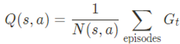
In summary, here is how Monte Carlo learning works — it estimates Q(s,a) , which is the Return of every action in every state by taking samples of complete episodes (terminal state reached). This means the Q(s,a) is updated at every complete episode. Recall in the MDP, Q(s,a) is the expected Return taking action aand state s:

However, in Monte Carlo learning, Q(s,a) is calculated as an approximate empirical mean where N(s,a) is the number of times that action ahas been taken at the particular state s, and G is the particular Return added, relative to the state s taking action a, at a particular episode:

However, by simply following this paradigm, we have to run many episodes, to the end perhaps, before we can approximate Q(s,a) , and then update the policy. Fortunately, we can do incremental updates with a simple trick:

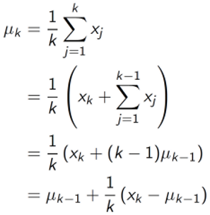
Hence, every incremental update becomes:

2.1 Algorithm for Monte Carlo Learning

So now we have a fundamental idea of how Monte Carlo learning works. Next, let us formulate the entire algorithm for Monte Carlo learning:

Initialization

• For each state s and action a , initialize arbitrary values for Q(s,a)
• Initialize N(s,a) = 0 for all s and a pairs. This counts the number of times action a has been taken at state s .
• Initiate uniform random policy π

Iteration For Every Episode

• Generate an episode following the ϵ-greedy policy π(a|s) w.r.t Q(s,a)
• For each pair of state s and action a appearing in the episode: Track the return G(s,a) for the occurrence of s and a
• Update N(s,a) = N(s,a) + 1
• Incremental update Q(s,a) = Q(s,a) + 1/N(s,a)*(G-Q(s,a))

Notice that in the above algorithm, Monte Carlo learning follows the Policy Evaluation and Policy improvement at every iteration (episode), which has similar paradigm to the Policy Iteration method in Dynamic Programming.

For a stationary MDP (transition probabilities and rewards do not evolve with time), the iteration can stop when there is little variation in Q(s,a), indicating that the optimal policy has been achieved.

For non-stationary MDP, we have to approximate the factor 1/N(s,a) with another constant α , since it is important to forget earlier episodes as the MDP evolves with time. In the case iteration should always continue, and the latest Q(s,a) should be taken for the best policy.

To illustrate, let us consider a more complex, but stationary, MDP:

Consider a 6x6 Gridworld, and initiate initial Q(s,a)=0 for all state-action pairs with uniform random policy, where states (1,1) and (1,6) are terminal states. Rewards is -20 all every state except the terminal states (1,1) with R=+100 and (1,6) with R=+60. For simplicity allow γ=1, and let transition be deterministic. Let the initial state randomly start at the bottom of grid (6,k).

import numpy as np
from tqdm import tqdm
from collections import defaultdict

class Gridworld:

    def __init__(self, size=6):
        self.size = size
        self.states = [(i, j) for i in range(1, size+1) for j in range(1, size+1)]
        self.terminal_states = [(1,1), (1,size)]
        self.actions = ['up', 'down', 'left', 'right']

    def step(self, state, action):
        if state in self.terminal_states:
            return state, 0
        i, j = state
        if action == 'up':
            i -= 1
        elif action == 'down':
            i += 1
        elif action == 'left':
            j -= 1
        elif action == 'right':
            j += 1

        i = max(1, min(i, self.size))
        j = max(1, min(j, self.size))
        next_state = (i, j)

        if next_state == (1,1):
            reward = 100
        elif next_state == (1,self.size):
            reward = 60
        else:
            reward = -20

        return next_state, reward

    def reset(self):
        bottom_states = [(6, j) for j in range(1, self.size+1)]
        return bottom_states[np.random.choice(len(bottom_states))]

def monte_carlo_control(env, num_episodes, discount_factor=1, epsilon=0.2):
    Q = defaultdict(lambda: defaultdict(float))
    returns_count = defaultdict(lambda: defaultdict(float))
    policy = defaultdict(str)

    for _ in tqdm(range(num_episodes)):
        state = env.reset()
        episode = []

        # Generate an episode
        while state not in env.terminal_states:
            probs = np.ones(len(env.actions)) * epsilon / len(env.actions)
            if Q[state]:
                best_action = max(Q[state], key=Q[state].get)
            else:
                best_action = np.random.choice(env.actions)
            probs[list(env.actions).index(best_action)] += (1.0 - epsilon)
            action = np.random.choice(env.actions, p=probs)
            next_state, reward = env.step(state, action)
            episode.append((state, action, reward))
            state = next_state

        # Update each Q(s,a) from an episode, in reverse order
        G = 0
        for t in reversed(range(len(episode))):
            state, action, reward = episode[t]
            G = discount_factor * G + reward
            returns_count[state][action] += 1
            Q[state][action] += (G - Q[state][action]) / returns_count[state][action]

    for state in Q:
        policy[state] = max(Q[state], key=Q[state].get)

    return Q, policy

env = Gridworld()
Q, policy = monte_carlo_control(env, num_episodes=1000000)

# Print the policy
for i in range(1, 7):
    for j in range(1, 7):
        state = (i, j)
        action = policy.get(state, "none")
        print(f"({i}, {j}): {action}", end=" | ")
    print()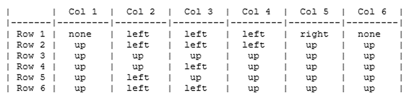

With the above Monte Carlo algorithm, we have shown that we can solve the MDP, by trial and error, without direct knowledge of the environmental dynamics (though we only considered deterministic transitions in the above 6x6 Gridworld example).

Note that, for every next iteration, we have run through the entire episode with the updated policy from the previous episode— that is we are continuously learning about the policy and improving it while implementing its latest version. We call this On-Policy Learning.

In the next section, we will understand another important learning paradigm that learns the optimal policy for an MDP, not by seeing how the target policy plays out each iteration, but instead by observing another policy in action — we call this Off-Policy Learning.

3. Off-Policy Monte Carlo Learning

You can think of Off-Policy Learning like this. Imagine you are learning how to cook, but you don’t want to start experimenting with food yourself for fear your initial products may not be good. As such, you learn by observing how another chef (maybe your grandmother) prepares the food repeatedly and then form your own critical opinion of what can be done — perhaps better — at each step of the preparation.

Hence, Off-Policy Learning is like learning from observing another human or other agents. Another application is perhaps training a robot to perform tasks at home. You would not want to let loose the robot learn from scratch by trial and error — who knows, it might damage itself or the environment in the process. Instead, you first programmed specific stochastic actions with regard to certain sensory inputs (states s ) it receives, and that forms the Behaviour Policy μ(a|s) . In this case, the robot then learns the Target Policy π(a|s) and its associated Q(s,a) values, while the robot is navigating episodes of trajectories based on Behaviour Policy μ(a|s) .

Another simple application would be to update a greedy policy while following an exploratory policy, which is the focus of this section — Off-Policy Monte Carlo Learning. This is almost similar to the On-Policy Monte Carlo learning algorithm — learning by trial and error through a series of episodes — that we have implemented in the previous section but with a little tweak.

3.1 Importance Sampling

To perform the Monte Carlo update, let us revisit the incremental update for Q(s,a) again.

Notice that we want to update the Q(s,a) based on the Target Policy π(a|s) . However, since each episode is run based on the Behaviour Policy μ(a|s) , we do not have the value of Return G for π(a|s) , as each Return G can only be computed based on μ(a|s) . Hence we need to do something else in order to get its estimate. This is where the mathematics of Importance Sampling comes in, as shown below:

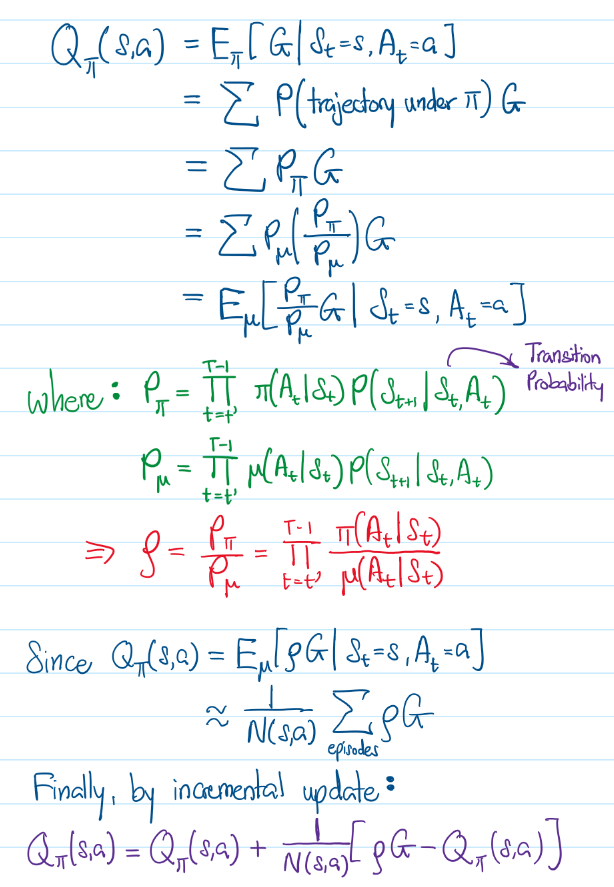
Note that the above term ρG is actually an estimate of Return G for π(a|s). As such, we can also approximate the factor 1/N(s,a) with another constant α. Applying these changes to the incremental update for Q(s,a) , we should be able to arrive at the Off-Policy Monte Carlo algorithm to learn the Target Policy π(a|s). Also, note that the above Return G in the equation above is computed based on the episode following a fixed Behaviour Policy, μ(a|s)which we can set with a uniform random policy.

We will illustrate the Off-Policy Monte Carlo algorithm based on the same 6x6 Gridworld MDP environment for the On-Policy Monte Carlo learning in the previous section:

def off_policy_monte_carlo_control(env, num_episodes, discount_factor=1):
    Q = defaultdict(lambda: defaultdict(float))
    returns_count = defaultdict(lambda: defaultdict(float))
    policy = defaultdict(str)

    for _ in tqdm(range(num_episodes)):
        state = env.reset()
        episode = []

        # Generate an episode using behavior policy (uniform random)
        while state not in env.terminal_states:
            action = np.random.choice(env.actions)  # Uniform random behavior policy
            next_state, reward = env.step(state, action)
            episode.append((state, action, reward))
            state = next_state

        G = 0.0  # Return
        W = 1.0  # Assume initial uniform random policy for Target policy, similar to behavior policy

        for t in reversed(range(len(episode))):
            state, action, reward = episode[t]
            G = discount_factor * G + reward

            # Update Q-value using ordinary importance sampling
            returns_count[state][action] += 1  # Count of returns for this state-action pair
            Q[state][action] += (W*G - Q[state][action])/ returns_count[state][action]

            # Update the target policy to be greedy
            if Q[state]:
                policy[state] = max(Q[state], key=Q[state].get)

            # Update importance sampling ratio
            if action == policy[state]:
                W *= 1 / (1/4)  # Target policy is deterministic (1), behavior policy is uniform random (1/4)
            else:
                W *= 0

    return Q, policy

4. Conclusion

Congratulations on reaching here! We have successfully implemented 3 Reinforcement Learning algorithms — one Model-based, one Model-free and another Model-free plus Off-Policy. They can be mainly applied to limited problems, though. For instance, in the Monte Carlo method, learning can only be updated at the end of every episode — this means that it is only an offline learning algorithm.

Monte Carlo learning may be great for applications like chess-playing. It’s only after every game, whether you or the observed agent (Off-Policy) won or lost, that upon reflection you will figure out better strategies to win the game next round. However, for situations where you need to update your Q(s,a) along the way before the episode ends, Monte Carlo is not very helpful.

Imagine when you are driving a car to the destination and along the way you nearly encounter a car crash. You could then make use of the experience to prevent another similar situation for the rest of the journey. However based on Monte Carlo learning, you would have crashed your car (your journey ended), before you would update your learning. That is impractical!

For problems that require online learning — or learning on the fly — we would have to look into temporal difference methods, such as SARSA and Q-Learning, and that would be our focus in the next article — Part 3. Hence, do check out the Part 3 here:

P.S: Some of the diagrams and equations used in this article are adapted from the free lecture slides by David Silver here.

Thanks for reading! If you have enjoyed the content, pop by my other articles on Medium and follow me on LinkedIn.

Support me! — If you are not subscribed to Medium, and like my content, do consider supporting me by joining Medium via my referral link.