
Regulate Your Regression Model With Ridge, LASSO and ElasticNet
What are regularization techniques and why do we use them? A Python sklearn example is provided.

Linear models have a wide appeal. Even with a basic understanding of Excel, it is possible to create a model that explains patterns in data. After attaching weights (coefficients) to explanatory variables (features), it is easy to assess the importance of individual variables when explaining the data. It is not surprising that linear models have been around for many decades, and are widely used throughout many domains, ranging from psychology to business administration and from machine learning to statistics.
Despite the superficial simplicity of linear models, many things can go wrong with them. Two particularly common problems are:
- Overfitting. Especially when having a large model with many explanatory variables, there is a tendency to fit the model to noise. The R² value may look great on training data, but the model will perform much worse on out-of-sample data.
- Multicollinearity: When designing explanatory variables, there is a chance they are correlated to each other (think the number of bedrooms and the area of a house). Strong multicollinearity makes assigning appropriate weights problematic.
If the aim is to make the model suitable for out-of-sample prediction there are solutions. (note: for statistical interference they make little sense) This article discussed three common regularization techniques, used to tackle the abovementioned problems and create more robust prediction models. If you just want to see the Python implementation (using sklearn), skip to the end.
Linear regression
When we discuss linear regression, we mean that the model is linear as a statistical estimation problem. A linear model can be as simple as y_salary=θ*x_years_experience+ϵ (with θ the weight, x the feature, y the dependent variable, and ϵ random noise) or as complicated as a high-degree multivariate polynomial. The basic concept remains the same though: the model is a linear combination of explanatory variables. We fit the model by estimating weights in a way that minimizes the error of the model.
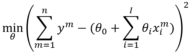
The most-used regression procedure (ordinary least squares or OLS) is intuitive and incorporated in many tools and libraries. For each data point, we can compute the difference (error) between the observation and the prediction by the model. By fitting the line such that the squared error is minimized, on average the model may explain each data point reasonably well.
Technical note: The assumption is that the model itself is correct, and that deviations of data points are the result of random noise.
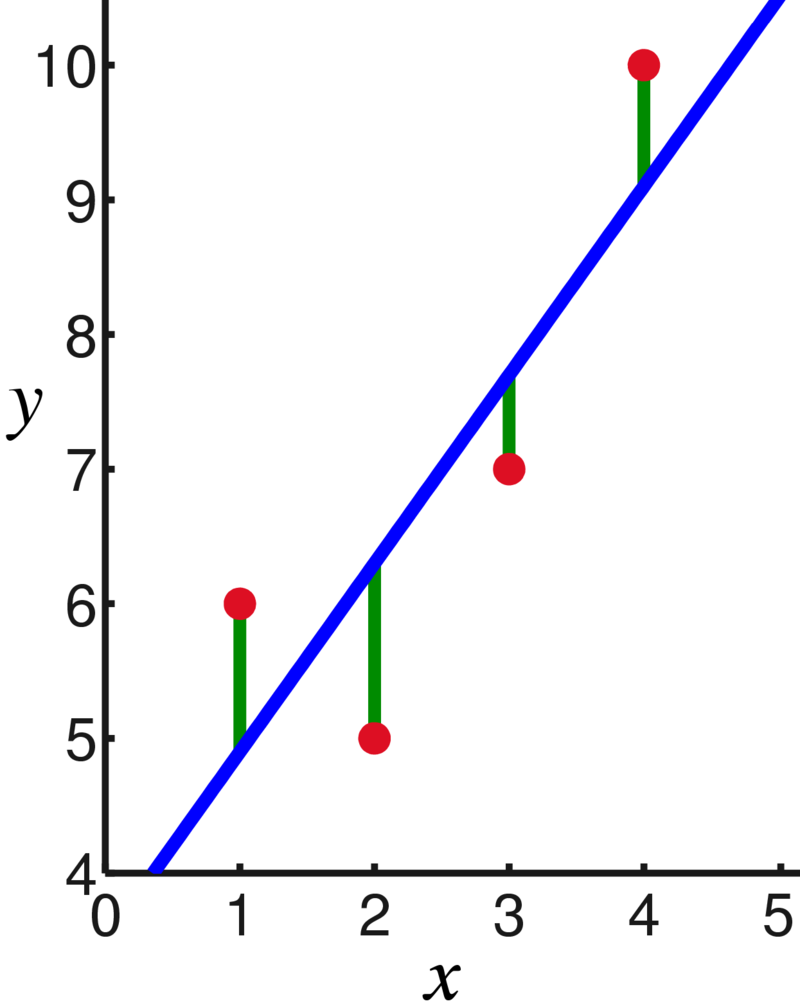
The case with a single explanatory variable (simple linear regression, y=θ*x+ϵ) is easy to visually. Typically, we deal with multiple variables though (multiple linear regression, defined by y=∑_i θ_i*x_i+ϵ). A large data set containing many (potential) explanatory variables is the most straighforward example.
In fact, we can design arbitrary complex features, e.g., when dealing with high-degree polynomials. Variables may be transformed (e.g., squaring a variable) or combined (e.g., multiplying two variables). It does not take much imagination to create arbitrarily large sets of features that result in very large regression models.
Although not the only potential cause, high-dimensional models (i.e., containing many features) tend to introduce the aforementioned multicollinearity and overfitting issues. Many features might (to a large degree) explain the same effect, or certain features might erroneously be assigned to explain certain outliers. Furthermore, a lot of features may have little to none explanatory power.
All these issues are not addressed by OLS regression, which simply minimizes the squared errors. Instead, we need to guide our model a bit, and that’s where regularization comes in.
Regularization
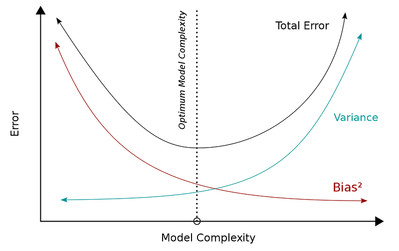
Statistical models harbor an innate tradeoff between bias and variance. In this context, bias describes errors stemming from erroneous assumptions, whereas variance refers to errors as a result of sensitivity to noise.
Although oversimplifying quite a bit here, high variance often goes hand in hand with multicollinearity and/or overfitting. Regularization aids in reducing the variance, at the cost of (intentionally) introducing some bias. Although potentially having a lower R² score than regular regression on the training set, the model may perform better on out-of-sample data when a more appropriate balance between bias and variance is struck.
This article discusses the three most common regularization techniques: LASSO, Ridge, and Elastic net.
LASSO regularization
LASSO is an abbreviation for “Least absolute shrinkage and selection operator”. The unabridged title is actually fairly descriptive: it aims to select the strongest explanatory variables by applying an absolute penalty. It is also known as L1 regularization.
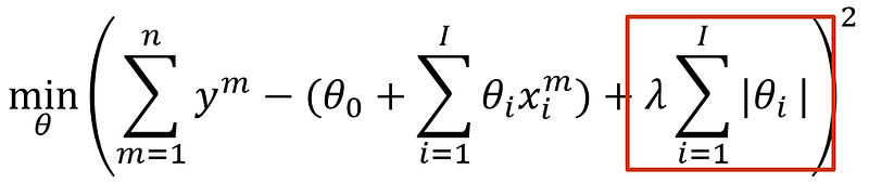
LASSO is mainly useful when dealing with large sets of explanatory variables, of which we suspect many have little relevance. LASSO can then be applied to set weights to 0 and whittle down our model to a smaller and more comprehensive one. The procedure can be performed iteratively (e.g., increasing λ with each step), gradually reducing the size of the model.
A potential disadvantage of LASSO is that it tends to select just a single variable out of a set of correlated ones. Although addressing multicollinearity, the model may also lose predictive power this way. Furthermore, when dealing with data sets characterized by many explanatory variables and only few data points (also know as the “large p, small n” case), LASSO will select at most n variables.
In summary, LASSO can be quite aggressive in sizing down regression models, and as such should be used with caution.
Ridge regularization

Although superficially looking similar to LASSO, ridge regularization — also Tikhonov- or L2 regularization — has a notably different effect. It also applies a penalty to the OLS formulation, but penalizes squared weights instead of absolute weights:
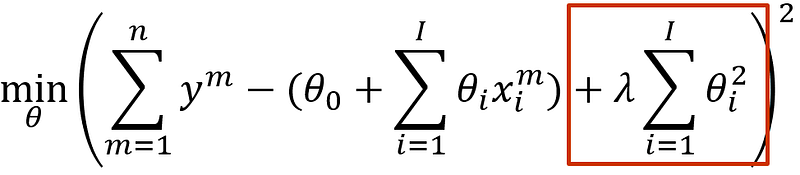
The effect is stronger than you might expect. Remind that 20²=40, 2²=4 and 0.2²=0.04. Thus; ridge severely penalizes large weights, but small weights are actually beneficial. Consequently, Ridge regularization tends to distribute many small (non-zero) weights across the spectrum of features.
You may imagine that a model with several very high weights responds sharply to changes in the corresponding variables. By distributing weights more evenly, ridge regularization yields a ‘smoother’ model, hence the name of the procedure.
Typically, we would use ridge regression when dealing with relatively few explanatory variables. Unlike LASSO, it does not help in feature selection. The main benefit of ridge regression is that it tends to reduce variance considerably.
Elastic net regularization
As with many things in life, balance is key. L1 and L2 penalties each have specific purposes, but sometimes we want a bit of both. More specifically, we might want to reduce the number of features, but also spread weights more robustly across the remaining features. This is what elastic net regularization does. It simply adds both L1 and L2 penalties with certain weights:
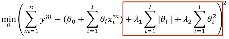
Note that λ_1 and λ_2 can be set by the user, enabling to balance L1 and L2. In the extremes, you can apply pure LASSO- or ridge regression. Ideally, elastic net regularization enables to select good features and create a robust model for them. However, it is also susceptible to the downsides of both LASSO and ridge. Naïve application of elastic net regularization can yield very poor results.
sklearn example
It’s always best to get some hands-on experience with modeling techniques, so I added a brief Python example using the sklearn library. The built-in California housing dataset contains 8 features (e.g., proximity to the ocean, number of bedrooms) and the median house price per district. Note that I just use the raw data set without any tuning effort or iterative procedure— surely you can do much better than this.
Actual improvements in out-of-sample predictions are out of scope here (i.e., the results are not great…), but the intended behavior is visible in the regression coefficients:
===No regularization===
Weights:
 [ 4.33102288e-01 9.32362843e-03 -1.00332994e-01 6.15219176e-01
 -2.55110625e-06 -4.78180583e-03 -4.29077359e-01 -4.41484229e-01]
MSE: 0.544
R²: 0.601

===LASSO regularization===
Weights:
 [ 1.45469232e-01 5.81496884e-03 0.00000000e+00 -0.00000000e+00
 -6.37292607e-06 -0.00000000e+00 -0.00000000e+00 -0.00000000e+00]
MSE: 0.974
R²: 0.286

===Ridge regularization===
Weights:
 [ 4.36594382e-01 9.43739513e-03 -1.07132761e-01 6.44062485e-01
 -3.97034295e-06 -3.78635869e-03 -4.21299306e-01 -4.34484717e-01]
MSE: 0.543
R²: 0.602

===Elastic net regularization===
Weights:
 [ 2.53202643e-01 1.12982857e-02 0.00000000e+00 -0.00000000e+00
 9.63636030e-06 -0.00000000e+00 -0.00000000e+00 -0.00000000e+00]
MSE: 0.786
R²: 0.424
We see that ridge regression makes small coefficients a little bigger. The R² is marginally better compared to standard regression; the mean-squared error is slightly smaller. LASSO and elastic net set many coefficients to 0 and performs notably poorly; apparently, many useful features have been eliminated.
The results illustrate that blindly applying regularization techniques not necessarily skyrockets your prediction performance; quite the opposite. The theoretical benefits of regularization are eminent, but proceed with caution.
Key takeaways
- Especially when dealing with large numbers of features (e.g., high-dimensional data), overfitting and multicollinearity can cause considerable problems in linear regression.
- Regularization techniques aid in creating more robust models by penalizing weight allocations, often resulting in better out-of-sample prediction when correctly applied. They are not suitable for statistical interference.
- Regularization penalties are added to the OLS regression function. Compared to OLS, they deliberately introduce bias in order to reduce variance, making the model less sensitive to noise and outliers.
- LASSO (L1) regularization penalizes the absolute sum of weights. Consequently, many weights are set equal to 0. LASSO is useful to select salient features out of large sets and create simpler models, but also may drastically reduce predictive power.
- Ridge (L2) regularization penalizes the squared sum of weights. The result is that it tends to distribute weights more evenly than OLS, being less sensitive to changes in certain features. It does not help in selecting features.
- Elastic net regularization combines both L1 and L2 penalties with certain weights. At its best, it yields compact and robust regression models, but it also has many potential downsides.
- Naïve applications of regularization techniques may considerably reduce the quality of a regression model. Often, iterative procedures and certain transformations are needed to get the best out of them.
Considering to apply regularization? Be sure to not make this common mistake:
Interested in regression? You might also want to read up on polynomial regression:


