
Deep Learning
Radial Basis Function Neural Network Simplified
A short introduction to radial basis function neural network

Radial basis function (RBF) networks have a fundamentally different architecture than most neural network architectures. Most neural network architecture consists of many layers and introduces nonlinearity by repetitively applying nonlinear activation functions. RBF network on the other hand only consists of an input layer, a single hidden layer, and an output layer.
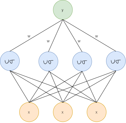
The input layer is not a computation layer, it just receives the input data and feeds it into the special hidden layer of the RBF network. The computation that is happened inside the hidden layer is very different from most neural networks, and this is where the power of the RBF network comes from. The output layer performs the prediction task such as classification or regression.
Input Layer
The input layer simply feeds the data to the hidden layers.
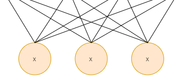
As a result, the number of neurons in the input layer should be equal to the dimensionality of the data. In the input layers, no computation is performed, as is the case with standard artificial neural networks. The input neurons are fully connected to the hidden neurons and feed their input forward.
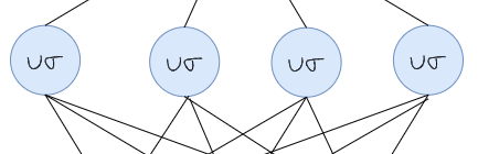
Hidden Layer
The hidden layer takes the input in which the pattern might not be linearly separable and transform it into a new space that is more linearly separable. The hidden layer has higher dimensionality than the input layer because the pattern that is not linearly separable often needs to be transformed into higher-dimensional space to be more linearly separable. This is based on Cover’s theorem on the separability of patterns, which states that a pattern that is transformed into a higher-dimensional space with nonlinear transformation is more likely to be linearly separable, therefore the number of neurons in the hidden layer should be greater than the number of the input neuron. With that said, the number of neurons in the hidden layer should be less than or equal to the number of samples in the training set. When the number of neurons in the hidden layer is equal to the number of samples in the training set, the model can be thought roughly equivalent to kernel learners such as kernel regression and kernel support vector machines.
The computations in the hidden layers are based on comparisons with prototype vectors which is a vector from the training set.
Each neuron in the hidden layer has a prototype vector and a bandwidth denoted by μ and σ respectively. Each neuron computes the similarity between the input vector and its prototype vector. The computation in the hidden layer can be mathematically written as follow:
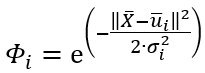
With:
- X bar as the input vector
- μ bar as the iᵗʰ neuron’s prototype vector
- σ as the iᵗʰ neuron’s bandwidth
- phi as the iᵗʰ neuron’s output
The parameters μ bar and σ are learned in an unsupervised way, for example using some clustering algorithm.
Output Layer
The output layer uses a linear activation function for both classification or regression tasks.
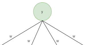
The computations in the output layer are performed just like a standard artificial neural network which is a linear combination between the input vector and the weight vector. The computation in the output layer can be mathematically written as follow:
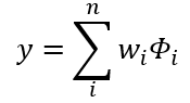
With:
- wᵢ as the weight connection
- phi as the iᵗʰ neuron’s output from the hidden layer
- y as the prediction result
The resulting prediction can be used for both classification or regression tasks, it depends on the target and loss function. The parameters w are learned in a supervised way such as gradient descent.
Although the output layer of RBF can be used as the final output, it is possible to stack RBF networks with other networks, for example, we can replace the output layer of the RBF network with a multilayer perception and train the network end-to-end.
Conclusion
The RBF network only consists of a single hidden layer that has its own way of computing the output. RBF network is based on the cover theorem, it casts the data into a higher-dimensional space by using its hidden layer, therefore the number of neurons in the hidden layer should be greater than the number of neurons in the input layer. The output layer uses a linear activation function or can be thought of without any activation function.


