
Quantum Computing (3) — — Quantum Annealing

Performing quantum computing involves understanding the basics of quantum mechanics and how it applies to computation. Quantum computing units, such as quantum annealers and quantum gates play a crucial role in quantum computing. These units operate on qubits, which are quantum versions of classical bits but can exist simultaneously in a superposition of multiple states, empowering quantum computing to surpass conventional supercomputers tremendously in computation speed and efficiency.
Wave Functions and Hamiltonian
As the qubits describing a system’s quantum state (or the quantum solution) are typically expressed as a wave function, it is essential to formulate a real-world problem in a way that quantum algorithms can solve. For example, factoring a large integer is a cryptographic problem in the real world. To solve this problem, which is intractable to conventional computers, one needs to translate the problem into one that a proper quantum algorithm can address.
Shor’s algorithm [1] for integer factorization is one such quantum algorithm. The algorithm manipulates the corresponding wave functions through certain quantum circuits to find the solution. One can leverage the quantum principles of superposition and entanglement to build Shor’s algorithm for integer factorization. Here, one doesn’t have to write a wave function explicitly for the problem. Instead, one can prepare a quantum state representing all possible superposition solutions. (I.e., the initial state is a superposition of all possible eigenstates of the wave function.) This is where the advantage of parallel computing is exploited.
A typical process of executing Shor’s Algorithm involves the following steps:
Initialization: Quantum registers are initialized in a superposition of all possible states, e.g., using Hadamard gates.
Modular exponentiation [2]: A wave function encoding the problem (e.g., modular exponentiation for factorization) is applied, which exploits quantum parallelism to evaluate the wave function for all input states simultaneously.
Quantum Fourier transform (QFT) [3]: Applied to the output register, the QFT helps find the period of the wave function, which is crucial for factoring. The QFT is where superposition plays a key role, transforming the quantum state into one where the periodicity of the wave function is encoded in the probabilities of the outcomes.
Measurement and classical post-processing: The final step involves measuring the quantum state, which collapses it to a specific outcome from which information about the solution can be extracted using classical algorithms.
Superposition allows quantum algorithms to process vast amounts of possibilities simultaneously. In Shor’s algorithm, superposition is used to prepare states and in the QFT to encode periodicity information.
Entanglement is used to create correlations between qubits. In Shor’s algorithm, the entanglement isn’t the primary focus. Still, it’s inherent in quantum operations that manipulate the state of multiple qubits, linking their information in ways that classical correlations cannot.
In this case, Shor’s algorithm doesn’t directly solve for a wave function, Ψ, for a Hamiltonian. Instead, it uses quantum states and operations to exploit quantum mechanical principles for computational purposes, primarily through the clever use of superposition and quantum interference. This empowers the algorithm to factor large integers, which is intractable for conventional supercomputers.
Quantum Annealing
Depending on the requirement details of solving for wave function Ψ in a Hamiltonian, quantum computing architectures are grouped into the quantum-annealer-based and the quantum-gate-based. Previous articles [4, 5] in this series dealt primarily with problems solvable with the quantum-gate-based approaches. There will be more such articles to come. However, this article focuses on the applications using the quantum-annealer-based approaches. This is because there is a set of problems (i.e., the optimization problems) that the quantum-annealer-based computers can easily address.
Quantum annealing is a quantum computing method used to find the global minimum of a problem by exploiting quantum mechanics principles like tunneling and superposition. It’s named “quantum annealing” in analogy to classical annealing, where a material is heated and then gradually cooled to remove defects.
Quantum annealing has demonstrated great potential in solving optimization problems, where the Hamiltonian encodes the problem to be solved. The system evolves to find the ground state corresponding to the optimal solution. Applications include improving machine learning, drug discovery, and a whole host of others, where it finds optimal solutions among a vast number of possibilities.
This article selects financial portfolio optimization as an example to illustrate how to set up an algorithmic framework to enable quantum approaches that find solutions much faster than classical algorithms.
Although quantum annealing is particularly suited for optimization problems, it has to be said that it is not universally the best approach; its effectiveness compared to gate-based quantum computing varies with the problem’s nature and the quantum annealer’s capability. Gate-based quantum computing offers a broader range of algorithms that can solve a wider variety of problems beyond optimization, including factoring and database searching, where it also promises substantial speedups over classical approaches.
An illustrative code for financial portfolio optimization
A financial portfolio optimization problem typically aims to allocate investments across a set of assets to maximize return for a given level of risk or minimize risk for a given level of return (e.g., using the mean-variance optimization model). The code below is a highly simplified example. It illustrates how to solve a financial portfolio optimization problem using quantum computing.
import numpy as np
import pandas as pd
from scipy.optimize import minimize

# Step 1: Define the problem
n_assets = 4
historical_returns = np.random.randn(252, n_assets)
expected_returns = np.mean(historical_returns, axis=0)
cov_matrix = np.cov(historical_returns.T)

# Step 2: Define the objective function
def portfolio_variance(weights):
    return weights.T @ cov_matrix @ weights
constraints = ({'type': 'eq', 'fun': lambda weights: np.sum(weights) - 1})
bounds = tuple((0, 1) for asset in range(n_assets))

# Step 3: Optimization
initial_guess = np.array([1./n_assets for _ in range(n_assets)])
opt_result = minimize(portfolio_variance, initial_guess, method='SLSQP', bounds=bounds, constraints=constraints)

# Step 4: Generate optimized financial portfolio
optimal_weights = opt_result.x
print("Optimal Portfolio Weights:", optimal_weights)
print("Expected Portfolio Return:", np.sum(optimal_weights * expected_returns))
print("Expected Portfolio Variance:", portfolio_variance(optimal_weights))
If one runs this code, they should be able to obtain their outputs in the following format:
Optimal Portfolio Weights: [0.26510454 0.24575885 0.26436336 0.22477325]
Expected Portfolio Return: 0.005439184214262248
Expected Portfolio Variance: 0.2511823629172556
Where 0.26510454, 0.24575885, 0.26436336, and 0.22477325 can be interpreted as that asset-1 should weigh c.a. 26.5%, asset-2 c.a. 24.6%, asset-3 c.a. 26.5%, and asset-4 c.a. 22.5% in the optimized 4-asset financial portfolio. The financial return of this portfolio is expected to be c.a. 0.54%, with the risk of not achieving this return being c.a. 25.1%.
Please note that this code does not truly optimize the financial portfolio; the code only serves to demonstrate the principle of quantum computation, as the historical returns fed into the calculation are randomized for easy illustrations. In addition, the numerical values of the output, Optimal Portfolio Weights, Expected Portfolio Return, and Expected Portfolio Variance, will change from one run to another since random functions are involved.
Notes on coding details
Step 1 of the code defines the problem. For easy illustration, the ‘n_assets = 4’ arbitrarily assumes the portfolio contains 4 assets. The ‘historical_returns = np.random.randn(252, n_assets)’ assumes historical returns being random for illustration purposes and arbitrarily sets trading days as 252. The ‘expected_returns’ and ‘cov_matrix’ denotes expected returns and covariance matrix.
Step 2 defines the objective function as minimizing the portfolio’s variance (risk). The ‘constraints’ and ‘bounds’ denote the constraints and boundary conditions (e.g., the sum of weights = 1 and weights ≥ 0).
In Step 2, the @ symbol is the matrix multiplication operator. It performs matrix multiplication between the arrays. The line, ‘return weights.T @ cov_matrix @ weights’, calculates the portfolio variance by multiplying the transpose of the weights vector, the covariance matrix (‘cov_matrix’), and the weights vector.
The line, ‘bounds = tuple((0, 1) for the asset in range(n_assets))’, generates a tuple of tuples, where each inner tuple is (0, 1). It represents the bounds for each asset’s weight in the portfolio, meaning each weight can vary between 0 and 1 (inclusive). The expression (0, 1) for the asset in ‘range(n_assets)’ creates an iterator that generates (0, 1) pairs ‘n_assets’ times. Wrapping this with ‘tuple()’ converts it into a tuple of these pairs, defining the optimization problem’s bounds.
Step 3 sets up the optimization mechanism. The ‘np.array([1./n_assets for _ in range(n_assets)])’ assumes equal allocation across the 4 assets as the initial state of the portfolio. The ‘_ (underscore)’ is a throwaway variable, which means its value is not intended to be used. It’s just a placeholder in loops where you don’t need to access the loop variable.
The expression ‘1./n_assets’ calculates the fraction 1/’n_assets’ and uses it to distribute the initial guess for the portfolio weights evenly among all assets. I.e., each asset is initially assigned the same weight, which is equal to the reciprocal of the total number of assets. The notation ‘1.’ ensures floating-point division, which is not strictly necessary if the division defaults to floating-point.
Using ‘1./n_assets’ is specific to the context of portfolio optimization and starts with an equal distribution of investment across all assets. This should be distinguished from the case of initializing quantum states, where a normalization coefficient of 1/sqr(2^m) is often used. This will be further discussed in the section, Realizing algorithmic steps physically.
Also, in Step 3, the ‘minimize()’ function is a general-purpose optimization function that attempts to find the minimum value of a function (in this case, ‘portfolio_variance’) given some constraints (‘constraints’), bounds (‘bounds’), and an initial guess (‘initial_guess’).
SLSQP stands for Sequential Least Squares Programming. It is an optimization algorithm that can handle both bounds and constraints. It’s particularly suited for nonlinear problems where the objective function and constraints are smooth functions. This step is used to find the weights that minimize the portfolio variance subject to the constraints (e.g., weights summing to 1 and each weight being between 0 and 1).
Step 4 Generates optimized financial portfolio and desired printouts. In the context of the ‘minimize()’ function, ‘opt_result’ is an object that contains the result of the optimization process. The ‘x’ attribute of this object stores the values of the variables (in this case, the portfolio weights) that minimize the objective function, given the specified constraints and bounds. Essentially, ‘opt_result.x’ is the solution to the optimization problem, representing the optimal weights for the portfolio.
Overall, the code above offers a simplified example of portfolio optimization, where the objective is to find the set of weights that minimizes the portfolio’s variance (risk), subject to constraints like the weights summing to 1. This code sets up a basic portfolio optimization framework using historical returns to calculate expected returns and the covariance matrix for a set of assets. The optimization aims to minimize the portfolio’s variance, subject to the constraint that the sum of the weights is 1 and all weights are non-negative, representing a proportion of the total investment in each asset.
Either quantum annealing or gate-based quantum computing solutions could replace the classical optimization part (Step 3: Optimization) in the code above. Quantum approaches can solve the portfolio optimization problem more efficiently by exploring the solution space more broadly and possibly escaping local minima better than classical methods.
Caveats
To solve a portfolio optimization problem using quantum annealing and leveraging quantum principles like tunneling, superposition, and entanglement, paying attention to the following coding aspects is often necessary:
· Define the portfolio optimization problem: Represent the portfolio’s expected return and risk (variance) and set your optimization goal, such as minimizing risk for a given return.
· Setting up the Hamiltonian: The key to this step is to encode the real-world problem (e.g., minimum variance in a financial portfolio optimization) into a quantum Hamiltonian (operator). This translates the financial problem into a quantum problem, where the Hamiltonian bridges the real-world requirements to the quantum wave functions. When the Hamiltonian operates on the wave functions, each quantum state wave function represents a possible portfolio allocation, and each state’s energy (eigenvalue) represents the portfolio’s performance (e.g., risks). The ground state wave function corresponds to the optimal solution of the real-world problem.
· Setting up the wave function: In setting up a wave function to describe the system (where the real-world problem stems from), it is critical to ensure that (1) the wave function contains an adequate number of qubits and (2) the wave function is initialized in a superposition state representing all possible solutions.
Lacking (1) will result in false optimal solutions, and lacking (2) will deny the computation from harvesting the benefits of superposition and entanglement. Preparation of the initial superposition state is often achieved by using specially designed quantum devices (e.g., quantum gates) that can engage multiple qubits simultaneously.
· Quantum annealing process: The core of this process is to gradually adjust the system from the initial Hamiltonian to the problem Hamiltonian (e.g., a specially designed Hamiltonian for financial portfolio optimization, in this case). This step involves carefully tuning the system’s parameters over time and is at the core of the quantum annealing.
This step is also where the quantum tunneling may take place. Quantum tunneling allows the system to transition through energy barriers instead of climbing over them, as in classical systems. This property helps the system skip local minima during annealing, potentially finding the global minimum more efficiently.
· Measurement: This is typically the last step of the quantum annealing process. When the system eventually settles into a state representing the ground state (i.e., the eigenstate with the lowest eigenvalue) of the problem Hamiltonian, the ground eigen wave function corresponds to the optimal solution.
Measurement is the quantum mechanical terminology that describes the action on a wave function by an operator, such as the problem Hamiltonian. The measurement collapses the system into a state representing an optimal (or near-optimal) portfolio allocation. For those who may not be familiar with relating quantum computation outcomes to real-world problems, seeking help to translate the measured quantum wave functions back to the classical solution (e.g., the optimal portfolio allocation) may be necessary.
Realizing algorithmic steps physically
An optimization challenge in our daily life may present itself as: “Should I ship this package by train along this long route or by ship directly?” or “What is the most efficient route for a traveler to visit the odd numbers cities on the city list?”
Physics can help solve these sorts of problems if one knows how to reframe them as energy minimization problems. A fundamental principle in physics is that everything tends to seek a minimum energy state. Phenomena such as objects sliding down hills and hot objects cooling down over time are well-known manifestations of this principle.
Quantum annealing leverages this principle and mimics the natural drive towards energy minimization to find “low-energy” states of a problem and, consequently, the optimal or near-optimal solution to the real-world problem. It enables quantum computing algorithms to tackle complex optimization problems by mapping them onto quantum systems, subsequently enabling them to evolve towards states with minimal energy.
A superposition wave function of a given number of qubits can typically be written as a linear sum of corresponding basis wave functions. Mathematically, this is described as being represented by a vector in Hilbert space, whereas Hilbert space is the mathematical framework that can describe a system’s quantum states.
Hilbert space is a vector space with an inner product, allowing for the description of superpositions and entanglements in quantum systems. Quantum computations use vectors in Hilbert space to represent the wave functions of the quantum system. Operations on these vectors correspond to transformations of the system.
For a financial portfolio optimization problem, both the initial Hamiltonian and the problem Hamiltonian must encode the portfolio’s configurations and associated costs (variances). The initial Hamiltonian might be simple, promoting an equal superposition state, while the problem Hamiltonian encodes the actual optimization problem, linking portfolio variances (e.g., cost or risk) to energy levels.
Gradual adjustment involves changing the system from the initial Hamiltonian and the problem Hamiltonian over time. This can be achieved, e.g., by using a schedule that ensures the system remains close to its ground state.
For the 4-assets portfolio optimization problem described in the code above, a proper wave function should contain a minimum of 4 qubits if each asset can opt to be either in or out of the portfolio. The initial wave function should look like the following,

In this expression, the |0001⟩, |0110⟩, |1101⟩, etc., are referred to as the basis wave functions (or the basis states) in ket notation.
For instance, if 0 is set to symbolize an asset being excluded from the portfolio, and 1 is set to symbolize an asset being included in the portfolio, then the basis wave function |0001⟩ (which is equivalent to |0⟩|0⟩|0⟩|1⟩ in this case) represents the basis wave function (i.e., the basis state) where the assets #1, #2, and #3 are not selected into the portfolio while only asset #4 is selected into the portfolio (i.e., the portfolio is entirely made of asset #4).
Similarly, the basis wave function |0110⟩ (which is equivalent to |0⟩|1⟩|1⟩|0⟩) represents the basis state where assets #1 and #4 are excluded from the portfolio while assets #2 and #3 are included in the portfolio (i.e., the portfolio is made of assets #2 and #3 only).
Overall, as each of the 4 assets has 2 possible states, included or excluded, the total number of combined states is 2⁴ = 16. Consequently, the Ψinit contains 16 terms (i.e., the 16 basis wave functions as shown in Eq. 1). In a quantum computation language, this can be restated as Ψinit being represented as a superposition of all possible states for a 4-qubit system, with each state corresponding to a different combination of the 4 assets being either included (1) or excluded (0) from the portfolio.
The 16 basis states are orthogonal in the Hilbert space, meaning their inner product (or overlap) is zero unless they are in the same state, in which case it is 1. This orthogonality ensures that they span the Hilbert space, allowing for the representation of any state of the system as a combination of these basis states.
The vector representation of Ψinit in the 16-dimensional Hilbert space is:

Eq. 1 and Eq. 2 are equivalent. They are just different representations of the same wave function. For a 4-qubit system, the normalization factor of the wave function is 1/sqr(16) = 1/4. One should avoid mistaking the normalization factor as 1/16 since, in quantum computing, the probability for the multiqubit state (the wave function) to collapse to a basis state is the square of its coefficient, i.e., (1/4)² in the case of Ψinit. In other words, the normalization factor should be determined by (Ψinit*)(Ψinit).
Generally speaking, for an m-assets portfolio, if each asset can be either in or out of the portfolio, one would need at least m qubits to represent all possible combinations. For an equally weighted superposition of m states, the normalization factor should be 1/sqr(2^m) to ensure that the total probability sums to 1. Thus, for a 4-qubit system with 16 basis states (2⁴ = 16), the normalization factor is 1/sqr(16) = ¼.
An equally weighted superposition of m states is an easily constructed state and is consequently widely used as a hypothetical initial state. For this reason, Eq. 1 is used to represent the initial wave function, Ψinit, for the 4-assets portfolio optimization problem discussed above.
One would need more qubits for more granular control over allocations (e.g., percentages). Ideally, one chooses the number of qubits based on the resolution of allocation they need. The number of qubits needed to represent an assets portfolio is dictated by the level of detail and the range of allocations that one wishes to represent.
The combination of the terms in the wave function should collectively represent the superposition of all possible states. In Hilbert space, the wave function is further simplified into a vector whose dimensionality is determined by the number of qubits (m) in the form of 2^m if each of the qubits has only 2 possible states (i.e., binary), illustrating the complex and multidimensional nature of quantum states.
At the end of the quantum annealing process, the wave function settles (or collapses) into its lowest-energy eigenfunction form. This eigenfunction still assumes the generic form of Eq. 1, but the coefficients in front of the 16 basis states are no longer uniformly ¼. Any of the 16 coefficients shall take a value in the 0 ≤ coefficient ≤ 1 range, with the sum of the squares of the 16 coefficients being 1.
For settling a single-qubit wave function into its lowest-energy eigen function by a quantum annealing process, the qubit can be physically represented by a spin or a magnetic dipole induced by a circulating current, as illustrated in Fig. 1.
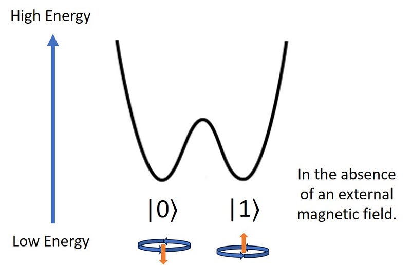
If each of the 4 assets in the financial portfolio is represented by a single-qubit wave function, |x⟩, then either x = 0 if the asset is excluded from the portfolio; or x = 1 if the asset is included in the portfolio. In other words, either |x⟩ = |0⟩ or |x⟩ = |1⟩.
Since the probability for |x⟩ = |0⟩ and the probability for |x⟩ = |1⟩ are assumed equal, i.e., 50%:50%, for the sake of convenience, the initial state wave function of the 4-asset-portfolio which is represented by a 4-qubit wave function, Ψinit, assumes the form of Eq. 1.
Suppose the influence of the financial market on the performance of an asset is encoded (e.g., into the Hamiltonian) as corresponding quantum annealing in the algorithm, and the quantum annealing is physically realized in a quantum computer, as indicated in Fig. 2, via applying a magnetic field to the spin or the magnetic dipole. In that case, the energy diagram for the single-qubit wave function will evolve, as illustrated in Fig. 2.
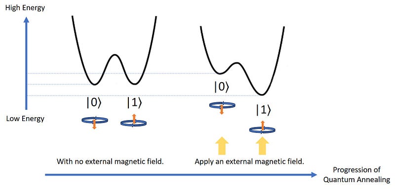
This diagram changes over time. As the quantum annealing progresses, the external magnetic field tilts the double-well potential, increasing the probability of the qubit ending up in the lower well. This energy minimization process continues until the respective qubit (i.e., the spin or magnetic dipole) reaches its lowest eigenvalue (i.e., energy in this case).
For a 4-qubit system representing a 4-assets portfolio, one needs to replace the single-qubit wave function, |x⟩, with the 4-qubit wave function, Ψinit. Fig. 3 is an energy diagram showing relative energy levels of 4-qubit basis functions in an external magnetic field. Fig. 3(a) shows the qualitative energy order in a homogeneous magnetic field, where energy levels of |1000⟩, |0100⟩, |0010⟩, |0001⟩ are clustered closely to each other and represented by |0001⟩; similarly, energy levels of |1001⟩, |0101⟩, |1010⟩, |0110⟩, |1100⟩, |0011⟩ are clustered closely to each other and represented by |0011⟩, etc., etc. Fig. 3(b) shows the qualitative energy order in a heterogeneous magnetic field.
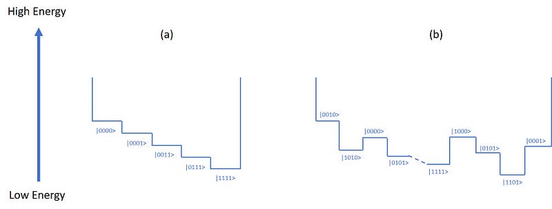
The best-performing portfolio is expected to be mapped to the 4-qubit eigen wave function with the lowest eigenvalue (i.e., energy in this case). In the case of Fig. 3(a), this eigen wave function is |1111⟩, as illustrated in Fig. 2 and Fig. 3(a). In the case of Fig. 3(b), this eigen wave function generally assumes the form of Eq. 3:

where 0 ≤ αijkl ≤ 1. This eigen wave function, Eq. 3, is not directly shown in Fig. 3. The details (i.e., the { αijkl }) of the Ψfinal (E = E0) are expected to change as the detail of the heterogeneous magnetic field changes.
The heterogeneous magnetic field is mapped to the problem Hamiltonian, which is, in turn, mapped to the financial market environment.
Readers are referred to Ref. [6] for more advanced reading on physical realizations of quantum annealing on quantum computers.
Concluding Discourse
The quantitative improvement of quantum annealing over classical methods depends on the problem’s complexity and the quantum hardware’s capability. While theoretical models suggest significant speedups for specific optimization problems, practical results highly depend on current quantum annealing technology advancements.
Recent advancements in quantum computing have led to developing a new architecture using fluxonium qubits, which achieves significantly higher fidelity in quantum operations. This architecture, which couples two fluxonium qubits with a transmon coupler, allows for single-qubit gate fidelity of 99.99% and two-qubit gate fidelity of 99.9%, surpassing the fidelity threshold needed for error-correcting codes. This breakthrough opens new possibilities for building fault-tolerant quantum computers and represents a significant step toward commercial and industrial quantum computing applications. [7]

References
[1] Wikipedia, Shor’s algorithm — Wikipedia
[2] Wikipedia, Modular exponentiation — Wikipedia
[3] Wikipedia, Quantum Fourier transform — Wikipedia
[4] Eric S. Shi, Quantum Computing (1) — — Error Mitigation Algorithm | Generative AI
[5] Eric S. Shi, Quantum Computing (2) — Superposition and Entanglement | Generative AI
[6] Wikipedia, https://en.wikipedia.org/wiki/D-Wave_Systems
[7] Adam Zewe, https://news.mit.edu/2023/new-qubit-circuit-enables-quantum-operations-higher-accuracy-0925)
Allow me to take this opportunity to thank you for being here! I would be unable to do what I do without people like you who follow along and take that leap of faith to read my postings.
If you like my content, please (1) leave me a few claps and (2) press the “Follow” button below my photo. I can also be contacted on LinkedIn and Facebook.
Brain-Computer Interfaces: The Next Frontier in Human Technology | Generative AI (medium.com)
Attention Mechanisms in Transformers | Artificial Corner (medium.com)
How an AI Model Acquires Its Writing Capability? | Artificial Corner (medium.com)

This story is published on Generative AI. Connect with us on LinkedIn and follow Zeniteq to stay in the loop with the latest AI stories. Let’s shape the future of AI together!


