
Quantum Computing (2) — Superposition and Entanglement
Building powerful circuits based on quantum mechanisms for new generation of parallel computing involves harnessing the unique properties such as superposition and entanglement of wave functions (i.e., the quantum states), where any change of one wave function instantly affects the probability distributions of all of its possible outcomes as well as those of its partner wave function(s), regardless of distance.
Superposition
Unlike classical bits, which can only be 0 or 1, qubits can simultaneously exist in a superposition of both states. This is often represented mathematically by the state vector:
|ψ⟩ = α|0⟩ + β|1⟩
where:
- |ψ⟩ represents the qubit’s state (i.e., wave function)
- α and β are complex numbers, with |α|² + |β|² = 1.
- |0⟩ and |1⟩ represent the basis states (i.e., the basis wave functions) of the qubit, analogous to 0 and 1 in classical bits.
Superposition can be visualized as a point on the Bloch sphere, where the poles represent |0⟩ and |1⟩, and any point on the sphere represents a superposition of both states:
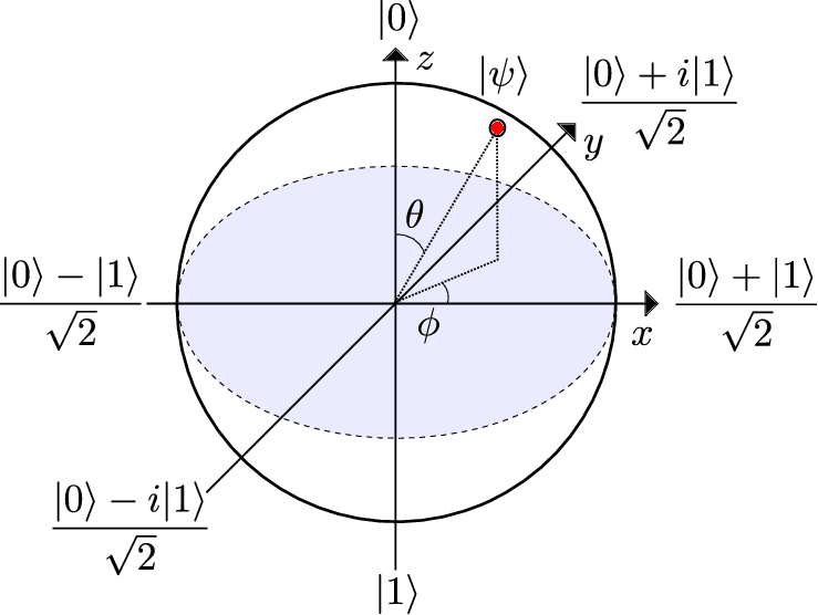
The probability of the qubit being in state |0⟩ or |1⟩ is determined by the absolute value of α and β, respectively.
Qubits’ ability to exist in superpositions allows for parallel processing. In a classical computer, bits must be processed one at a time. But in a quantum computer, a single qubit can simultaneously represent multiple states (in the form of superposition). This allows quantum computations to be performed simultaneously on all possible output states of a single input state, leading to a significant increase in computation speed.
For example, a classical computer trying to factor a large number would need to try different factors one by one. But a quantum computer could potentially factor the number much faster by exploring all possible factors simultaneously. (See section “Entanglement of Multi-qubit States” for more discussions and examples.)
Entanglement
Entanglement is a phenomenon where two or more qubits become linked in a way that their fates are intertwined, regardless of physical separation. This means that the state of one qubit is correlated with the state of the other(s), even when they are far apart.
For example, consider two entangled qubits in the state:
|ψ⟩ = (|00⟩ + |11⟩) / √2
Here, the two qubits are in a superposition of being both 0 and 1, but they are also entangled in such a way that if you measure the first qubit and find it to be 0 (or 1), you will instantly know that the second qubit must be 0 (or 1), too (and vice versa).
Entanglement, i.e., states of different qubits entangling with each other and exhibiting strong correlations, is a key resource for quantum computation and enables powerful algorithms that are impossible with classical computers.
Case Analysis of a Quantum Computing Code
The following short Cirq code is put together for this article. It serves to illustrate how the phenomena of quantum superimposition and entanglement can be simulated in a classical computer and, in turn, provide guidance to the architectural design of various configurations of gates and circuits for quantum computations.
import cirq
q0 = cirq.GridQubit(0, 0)
q1 = cirq.GridQubit(1, 0)
circuit = cirq.Circuit(
    cirq.H(q0),
    cirq.CNOT(q0, q1)
)
simulator = cirq.Simulator()
result = simulator.simulate(circuit)
print(result.final_state_vector)
circuit.append(cirq.X(q0))
result = simulator.simulate(circuit)
print(result.final_state_vector)
Expanded notes for the code above
Line 1: Imports the Cirq library for quantum circuit construction and simulation. (Note: Cirq is an open-source framework for NISQ computers.)
Lines 2–3: Create two qubits, q0 and q1, to represent quantum bits. For instance, GridQubit(0, 0) creates a qubit object in a 2D grid representation, in which (0, 0) specifies its coordinates on the grid, like a chessboard. Similarly, GridQubit(1, 0) creates another qubit object, and the (1, 0) specifies its coordinates.
Lines 4–7: Entangle the qubits (i.e., the wave functions) as follows.
- The H(q0) applies a Hadamard gate (H) to the |q0⟩ wave function (i.e., the q0 qubit) and transforms the qubit’s state to an equal superposition of |0⟩ and |1⟩, represented as: |ψ⟩ = 1/√2 (|0⟩ + |1⟩). Generally, a superposition of |0⟩ and |1⟩ can be expressed as |ψ⟩ = α|0⟩ + β|1⟩, where If β = 0, |ψ⟩ = α|0⟩; if α = 0, |ψ⟩ = β|1⟩.
- Assuming that the two inputs are |ψ1⟩ = α1|0⟩ + β1|1⟩ and |ψ2⟩ = α2|0⟩ + β2|1⟩, the cirq.CNOT(q0, q1) function entangles |ψ1⟩ (written as |q0⟩, the control qubit, in the code) and |ψ2⟩ (written as |q1⟩, the target qubit, in the code) using a controlled NOT (CNOT) gate.
- If the control qubit |ψ1⟩ is in |0⟩ (i.e., |ψ1⟩ = |q0⟩ = |0⟩), by definition, the target qubit remains unchanged. Therefore, the output would simply be |ψ2⟩ = b(α2|0⟩ + β2|1⟩), in the single-qubit expression.
If the control qubit |ψ1⟩ is in |1⟩ (i.e., |ψ1⟩ = |q0⟩ = |1⟩), by definition, the target qubit flips. Therefore, the output would be |ψ2⟩ = α2|1⟩ + β2|0⟩ since the CNOT gate acts as a controlled NOT (flip) operation. When the control is |1⟩ (meaning “flip if true”), it flips the target state.
Lines 8–9: Create a Cirq simulator and simulate the circuit to obtain the final state vector, representing the entangled state of the qubits.
Line 10: Prints the outcomes of executing lines 8–9 to reveal the entanglement.
Line 11: Applies an X gate (X) to |q0⟩. This is a single-qubit operation. This, in combination with line 12, reveals how a change in one qubit affects the other due to entanglement, demonstrating a principle behind parallel quantum computation.
Line 12: Re-simulates the circuit to observe how the operation on |q0⟩ affects both qubits due to entanglement, showcasing parallel computation.
Line 13: Prints the final state vector of the qubits after the operation on |q0⟩ to visualize the entanglement and parallel computation.
Upon successful execution of the above snippet, the first printout should read like
[0.5+0.j, 0.5+0.j, 0.5+0.j, 0.5+0.j]
This is in vector expression notation, representing a vector with four elements, each being in the form of a complex number 0.5+0.j. In other words, it represents an equal superposition of all four possible states (i.e., |00⟩, |01⟩, |10⟩, |11⟩) and indicates entanglement.
Here, the vector expression notation is commonly used as a shorthand for the following ket notation,
|ψ(1st)⟩ = (0.5+0.j)|00⟩ + (0.5+0.j)|01⟩ + (0.5+0.j)|10⟩ + (0.5+0.j)|11⟩
= 0.5|00⟩ + 0.5|01⟩ + 0.5|10⟩ + 0.5|11⟩.
Here, the amplitudes (i.e., the coefficients in front of the basis vectors) are in the form a+jb, where a = 0.5, b = 0, and the “j” represents the imaginary unit, often denoted as “i” in other contexts.
The second printout (after X gate) should read like
[0.5+0.j, -0.5+0.j, -0.5+0.j, 0.5+0.j]
which reveals that the X gate flips |q0⟩’s state and affects |q1⟩ accordingly. The amplitudes of |01⟩ and |10⟩ states are now negative, representing the change.
The outputs differ because the X gate changes the qubits’ state, and the simulator recalculates the final state vector. In the more commonly seen wave function form (ket notation), it can be expressed as
|ψ(2nd)⟩ = (0.5+0.j)|00⟩ — (0.5+0.j)|01⟩ — (0.5+0.j)|10⟩ + (0.5+0.j)|11⟩
= 0.5|00⟩ — 0.5|01⟩ — 0.5|10⟩ + 0.5|11⟩.
Key learnings from the case analysis
Cirq simulates quantum behavior but doesn’t fully replicate it. This simulation exemplifies how manipulating a single qubit in an entangled pair can simultaneously influence the other qubit, even without directly operating on it — — a key feature of quantum parallelism.
Actual quantum computers are needed to fully realize the benefits of quantum entanglement and achieve true parallel computation. Simulators can only approximate the behaviors. The above code provides a basic example of quantum entanglement in Cirq. Real-world quantum algorithms often involve more complex circuits and operations.
Understanding superposition, entanglement, measurement collapse, and quantum gates is crucial for harnessing the power of parallel computing in quantum circuits. By analyzing the state vectors, we can gain insights into the potential computational paths and the corresponding probabilities, paving the way for more powerful quantum algorithms.
Identification of Entanglement
Taking the CNOT gate as an example, the output state can be either entangled or not entangled, depending on the initial α1, β1 values of the |ψ1⟩ = α1|0⟩ + β1|1⟩, as well as the initial α2, β2 values of the |ψ2⟩ = α2|0⟩ + β2|1⟩. Entanglement must have occurred if the state of one qubit can no longer be described independently of the other in the output.
Mathematically, the occurrence of quantum entanglement can be identified either by inspecting the Schrödinger equation or by calculating the Schmidt coefficients, among other methods (e.g., the von Neumann entropy). These methods can be used in complement to one another.
The Schrödinger equation method
If the combined state can be written as a product of individual qubit states (e.g., |ψ1⟩ ⊗ |ψ2⟩), it’s not entangled. If it cannot be factored this way, it’s entangled.
The mathematical expression of the above statement is: If
iħ ∂|ψ⟩/∂t = H|ψ⟩ = |ψ1⟩ ⊗ |ψ2⟩
then |ψ⟩ is not entangled, where i is the imaginary unit, ħ is the reduced Planck constant, ∂|ψ⟩/∂t is the partial derivative of the wavefunction with respect to time, H is the Hamiltonian operator, representing the total energy of the system, |ψ⟩, |ψ1⟩, and |ψ2⟩ are the wavefunctions.
Schmidt coefficient method
This method decomposes the quantum state into a product of single-qubit states with non-zero Schmidt coefficients. As any bipartite state can be written as a sum of products of orthogonal states,
|ψ⟩ = ∑λij|ai⟩ ⊗ |bj⟩
where i, j, and ij are subscriptive indices. The non-zero coefficients signify entanglement. This is equivalent to saying that if you calculate the Schmidt coefficients of the quantum state and you obtain non-zero coefficients, λij, for multiple terms, then the quantum state is already entangled.
Entanglement of Multi-qubit States
Two-qubit state
If a single-qubit superposition state, |ψ1⟩ = α1|0⟩ + β1|1⟩ interacts with another single-qubit superposition state, |ψ2⟩ = α2|0⟩ + β2|1⟩, the outcome is, by definition, the tensor product of the two original states,
|ψ⟩ = |ψ1⟩ ⊗ |ψ2⟩ = (α1|0⟩ + β1|1⟩) ⊗ (α2|0⟩ + β2|1⟩)
= α1α2|00⟩ + α1β2|01⟩ + β1α2|10⟩ + β1β2|11⟩.
Generally speaking, such an interaction may create entanglements via correlated terms where the measurement of one qubit instantly determines the state of the other, as discussed in the section “Identification of Entanglement” above.
The Bell states describe the maximally entangled states of two qubits among all possibly entangled two-qubit wave functions. With the ket vector notation, the Bell states can be written as follows,
|Φ+⟩ = (|00⟩ + |11⟩) / √2
|Φ-⟩ = (|00⟩ — |11⟩) / √2
|Ψ+⟩ = (|01⟩ + |10⟩) / √2
|Ψ-⟩ = (|01⟩ — |10⟩) / √2.
Using the criteria stated in the section of “Identification of Entanglement”, one can easily verify that each and every one of the Bell states, e.g., (|(00) + (11)⟩)/√2, is indeed an entangled state, as it cannot be written as a simple product of single-qubit states.
Diagrammatically, entanglement can be visualized using the Bell state diagram. A Bell state diagram for either the |Φ+⟩, |Φ-⟩, |Ψ+⟩, or |Ψ-⟩ wave function consists of a set of four possible Bell states (i.e., |00⟩, |01⟩, |10⟩, and |11⟩). Here, the points representing the qubits on their respective Bloch spheres wouldn’t be independent. They would be linked by a specific geometric relationship, reflecting the correlations imposed by entanglement.
The Bell states are a set of fundamental examples of quantum entanglement, where the two qubits are inextricably linked, even if they are physically separated by a large distance. This unique type of correlation, showcasing quantum entanglement, cannot be replicated in classical computing. Entanglement is a subtle concept, but it’s at the heart of quantum computing’s potential power. It allows for computations that are impossible in the classical world.
On the other hand, it’s crucial to remember that not all states that appear factorizable are necessarily unentangled. For this reason, identifying and manipulating all kinds of entangled states remains a challenge in quantum information science.
Three-qubit state
By analogy, the mathematical expression of the three-qubit interaction can be written as
|ψ⟩ = (α1|0⟩ + β1|1⟩) ⊗ (α2|0⟩ + β2|1⟩) ⊗ (α3|0⟩ + β3|1⟩)
= α1α2α3|000⟩ + α1α2β3|001⟩ + α1β2α3|010⟩ + α1β2β3|011⟩
+ β1α2α3|100⟩ + β1α2β3|101⟩ + β1β2α3|110⟩ + β1β2β3|111⟩
Where each term represents a possible combination of individual qubit states, with their corresponding amplitudes.
From the discussions above, one can observe that superposition and entanglement enable the computation power of a quantum computer to increase exponentially as the number of interacting qubits increases linearly. By entangling 2 qubits (i.e., 2 wave functions), a single computation can access 4 (i.e., 2²) interlocked solutions simultaneously. By entangling 3 qubits (i.e., 3 wave functions), a single computation can access 8 (i.e., 2³) interlocked solutions in one go.
Mathematically, the parallel processing capability can be quantified using the concept of tensor product dimension. The dimension of the multi-qubit entangled wave function (|ψ⟩) is the product of the individual qubit dimensions, scaling up exponentially as 2^n, where n is the number of the involved individual qubits (i.e., wave functions).
By manipulating 1 qubit, you can essentially explore all the possible solutions in one go, achieving massive parallel processing power. In other words, adding more qubits through entangling operators (e.g., gates) will allow for parallel processing over larger numbers of computational trajectories, which are impossible for classical computers.
Classical computers operate on Boolean logic and algebra, and their computational power increases proportionally with the number of gates (or transistors) in the system. I.e., in a classical computer, the computational power increases linearly in tandem with the gates in the system.
How to Construct Entangled States
Entangled states can be created through various techniques, including (1) Direct interaction — bringing two qubits close together and allowing them to entangle; (2) Controlled gates — applying specific quantum gates to pre-prepared qubits to entangle them in a controlled manner; (3) Resource states — using preexisting entangled states as resources to create new entangled states.
Entanglement is a powerful resource that allows quantum computers to perform calculations beyond the reach of classical computers. It unlocks new ways of processing information and opens doors to groundbreaking discoveries in various fields.
Entanglement based algorithms
Entanglement allows qubits to share information instantaneously, regardless of distance, leading to parallel processing capabilities beyond classical computers. This, in turn, enables promising/efficient algorithmic solutions for seemingly intractable problems like (1) Breaking down large numbers into prime factors (i.e., integer factorization), which is crucial for cryptography; (2) Searching for a specific element in an unsorted database (e.g., Grover’s algorithm), which promises quadratic speedup compared to classical algorithms; (3) Correcting errors in quantum computations more efficiently than classical methods (i.e., quantum error correction).
Source of computation power
The maze below can help one visualize the supremacy of parallel quantum computing over the concurrent processing achievable with classical computer CPUs.
This maze has 25 T-junctions (i.e., 25 fork points where every incoming path is split into 2 new outward paths). For a classical computer, the typical approach to finding the correct path to navigate across the maze is to calculate and register all decisions made at each of the T-junctions along every forward path branch. For a simple maze, as shown above, there are 28 unique paths, each with 1 to 12 T-junctions.
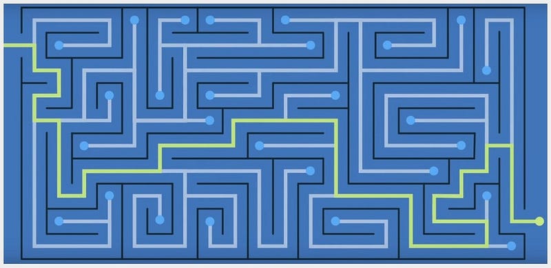
If one counts the T-junctions contained in each of the 28 paths sequentially, from the left edge of the maze toward the right edge, he obtains the following list, in the form of Route # (T-junctions contained): Route 1 (1); Route 2 (3); Route 3 (3); Route 4 (4); Route 5 (4); Route 6 (2); Route 7 (5); Route 8 (4); Route 9 (9); Route 10 (9); Route 11 (9); Route 12 (7); Route 13 (6); Route 14 (5); Route 15 (10); Route 16 (9); Route 17 (5); Route 18 (5); Route 19 (11); Route 20 (11); Route 21 (12); Route 22 (12); Route 23 (11); Route 24 (12); Route 25 (11); Route 26 (8); Route 27 (8); Route 28 (11).
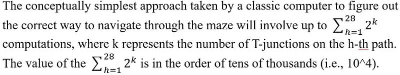
This exhaustive approach starts each trial from the very beginning of the journey (i.e., from the entrance point located at the north-west corner of the maze). Using a classical computer equipped with machine learning (ML), one can possibly reduce this value by an order of magnitude (i.e., to the level of 10³).
For a quantum computer, only 1 computation is needed, instead of c.a. 10⁴ computations by a classical computer or 10³ computations by a classical computer equipped with ML algorithms. The quantum computer will handle this problem as follows.
1. At each fork point, the quantum computer will entangle the input state (i.e., the multi-qubit wave function incoming to the fork point) with a new qubit (e.g., as a control qubit or wave function) via. a split operator (gate).
2. Each of all individual qubits remains as |0⟩ (i.e., a three-qubit wave function remains as |000⟩ and a five-qubit wave function as |00000⟩, and etc.) until the last one flips to |1⟩ when it hits a dead end (i.e., |000⟩ flips to |001⟩, |00000⟩ flips to |00001⟩, and etc.).
3. The entanglement among the qubits enables the quantum computer to identify the correct path (i.e., the green-colored path in the above maze) and navigate through the maze in only 1 attempt since the correct path features an all zero 11-qubit wave function, i.e., the |00…00⟩ with eleven 0’s, (consistent with having encountered no dead end upon passing all 11 T-junctions along the green-colored path and hence no flip form |0⟩ to |1⟩ in its wave function).
Typically, when attempting to factor a large integer, a classical computer would need to try different factors one by one. Yet, a quantum computer could potentially factor the integer much faster by exploring a huge number (if not all) of possible solutions in one go, and hence solve problems intractable to classical computers.
For example, the best-known classical algorithm for factoring a large integer is the General Number Field Sieve (GNFS). GNFS has a running time complexity in the neighborhood of O(n² (log n)²) where n is the number of bits in the integer. For a 256-bit integer, estimates suggest GNFS would take roughly 10¹⁴ years on even the most powerful classical supercomputers currently available. This exceeds the estimated age of the universe, which is around 13.8 billion years!
On the contrary, by leveraging the principles of quantum superposition and entanglement, Shor’s algorithm has a running time complexity of O((log n)³ ) which translates to roughly 23333 operations for a 256-bit integer.
The improvement is monumental. While GNFS requires an astronomical 10¹⁴ years on classical supercomputers, Shor’s algorithm could potentially complete the factoring in a few seconds on a large-scale quantum computer!
Quantum Modelling and Parallel Quantum Computing
Quantum algorithms are designed using a combination of quantum mechanics principles, mathematical tools, and operator theory. They involve constructing specific quantum circuits with devices like CNOT, Hadamard, and phase-shift gates to manipulate qubits according to the desired algorithm. Implementation involves specialized quantum hardware like superconducting qubits, trapped ions, neutral atom arrays, or photonic qubits, which have shown promise for building powerful quantum computers.
The key to parallel computing lies in the expansion of this entangled wave function. Each term in the combined wave function typically represents a path or computational trajectory for all involved qubits simultaneously. Manipulating just one qubit can effectively launch multiple computations on all possible combinations of states for all qubits. This is the essence of quantum parallelism enabled by entanglement.
As a crucial resource for quantum computation and an enabler of powerful algorithms, entanglement allows for parallel processing on a massive scale. The ability to perform parallel operations unlocks the potential for solving certain problems exponentially faster than classical computers.
However, quantum entanglement is a delicate phenomenon, and maintaining its coherence is crucial for successful parallel computations. Building large-scale quantum circuits with high-fidelity entanglement remains an ongoing challenge in the field. Understanding wave functions, their decoherence, and the design of quantum gates is crucial for comprehending quantum computation.
Potential Applications of Quantum Computing (Examples)
Molecular simulation
Consider two molecular isomers, A and B, with overlapping energy levels. Classically, determining the optimal reaction pathway for the interconversion between A and B would require simulating each of the possible intermediate steps sequentially, an exponentially complex task.
Using quantum programming, one can create an entangled state representing both molecular isomers in the initial states. Applying specific quantum gates manipulates the entanglement, effectively simulating all reaction pathways simultaneously. Measuring both the intermediate states and the final states reveals the probability of observing either A or B at a specific point along the reaction path, providing vital insights into the most likely reaction outcome under a given reaction thermodynamic/kinetic condition.
Quantum financial modelling
Imagine a portfolio optimization problem requiring analysis of a vast financial market dataset under various economic scenarios. Classically, evaluating each of the individual scenarios would be computationally prohibitive.
Using quantum algorithms, one can create an entangled state representing the various market variables and factors. Employing specialized quantum gates, one can manipulate this entangled state to explore all possible scenarios of the portfolio performance simultaneously. Measuring the final entangled state provides probabilities of different portfolio outcomes under each scenario, enabling efficient optimization strategies.
Drug discovery
The serendipitous nature of traditional drug discovery, characterized by laborious synthesis and testing cycles, hinders the efficient development of novel therapeutics. Quantum computing, by harnessing the unique properties of qubits, can precisely simulate the quantum mechanics of molecular docking, unveiling the intricacies of ligand-protein interactions with exceptional fidelity.
This capability paves the way for the design of drugs with tailor-made properties, optimized for binding affinity, specificity, and efficacy. As quantum algorithms and hardware continue to evolve, their role in drug discovery will likely extend beyond virtual screening, enabling researchers to fine-tune lead compounds at the atomic level and usher in a new era of precision therapeutics.
Materials science
The limitations of classical computational methods have long hampered the systematic design of materials with bespoke properties. However, leveraging the principles of superposition and entanglement, quantum computers can efficiently simulate the complex multi-electron interactions within materials, providing unparalleled insights into their fundamental properties. This capability enables researchers to explore vast chemical and structural landscapes, guiding the deliberate synthesis of materials with tailored electronic, optical, and mechanical characteristics. As quantum algorithms continue to evolve, their role in materials design is poised to transcend rudimentary prediction and usher in an era of precise atomic-level engineering.
Concluding Discourse
While the current state of quantum computing unveils a vista of groundbreaking applications across diverse domains, it represents a nascent step into the enigmatic realm of quantum mechanics. Further exploration of this fundamental framework and its transformative power promises to reshape numerous scientific and technological disciplines. As we continue to explore the intricate quantum phenomena and harness their computational prowess, we stand poised to witness a paradigm shift of unprecedented magnitude, reshaping our understanding of the universe and unlocking a future brimming with unimaginable possibilities.
Allow me to take this opportunity to thank you for being here! I would be unable to do what I do without people like you who follow along and take that leap of faith to read my postings.
If you like my content, please (1) leave me a few claps and (2) press the “Follow” button below my photo. I can also be contacted on LinkedIn and Facebook.
Quantum Computing (1) — — Error Mitigation Algorithm | Generative AI
Brain-Computer Interfaces: The Next Frontier in Human Technology | Generative AI (medium.com)
Attention Mechanisms in Transformers | Artificial Corner (medium.com)
How an AI Model Acquires Its Writing Capability? | Artificial Corner (medium.com)

This story is published on Generative AI. Connect with us on LinkedIn and follow Zeniteq to stay in the loop with the latest AI stories. Let’s shape the future of AI together!
