
QRNN: A Potential Competitor to the Transformer
Training Faster RNNs with Quasi-RNN

Recurrent Neural Networks (RNNs) have been in the sequence modeling business for a long time. But RNNs are slow; they process one token at a time. Moreover, the recurrent architecture adds a limitation of fixed-length encoding vectors for the complete sequence. To overcome these issues, architectures like CNN-LSTM, Transformer, QRNNs burgeoned.
In this article, we’ll be discussing the QRNN model proposed in the paper, “Quasi-Recurrent Neural Networks.” It is essentially an approach for adding convolution to recurrence and recurrence to convolution. You will get this as you proceed through the article.
Long Short-Term Memory (LSTM)
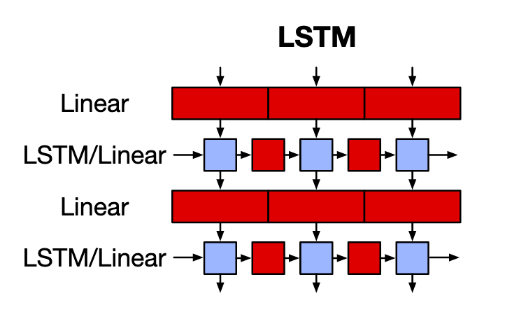
LSTM is the most well-known variant of RNNs. The red blocks are linear functions or matrix multiplications, and the blue ones are parameter-less element-wise blocks. An LSTM-cell applies gated functions (input, forget, output) to obtain the output and a memory element called the hidden state. This hidden state contains contextual information of the entire sequence. Since a single vector encodes the complete sequence, LSTMs cannot remember long-term dependencies. Moreover, the computation at each timestep is dependent on the hidden state of the previous timestep, i.e., LSTM computes one timestep at a time. Hence, the computations cannot be done in parallel.
Colah’s Blog is, by far, one of the best explanations for RNNs (in my opinion). Consider giving it a read if you’re interested in knowing the math behind LSTM.
Convolutional Neural Network (CNN)
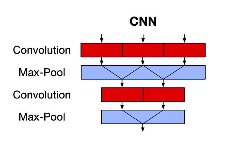
CNN, on the other hand, captures spatial features (mostly used in images). The red blocks are convolution operations, and blue blocks are parameter-less pooling operations. CNNs use kernels (or filters) to capture correspondence between features using a sliding window. This overcomes the fixed-length hidden representation (and thus, the long term dependency issue) as well as the lack of parallelism limitation of the RNNs. But, CNNs show no regard to the temporal nature of a sequence, i.e., time invariance. The pooling layers simply reduce the dimensionality of the channels without considering the sequence order information.
A Guide to Convolution Arithmetic for Deep Learning is one of the best papers on convolution operations involved in DL. Worth a read!
Quasi-Recurrent Neural Networks (QRNN)
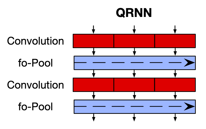
QRNN addresses the drawbacks of both the standard architectures. It allows parallel processing and captures long term dependencies like CNN, and also allows the output to depend on the order of tokens in the sequence like RNN.
So, to start with, the QRNN architecture has 2 components corresponding to the Convolutional (red) and Pooling (blue) components in CNN.
The Convolutional Component
The convolutional component operates with the following:
- The input sequence of shape: (batch_size, sequence_length, embed_dim)
- A ‘bank’ of ‘hidden_dim’ kernels of shape: (batch_size, kernel_size, embed_dim) each.
- The output is a sequence of shape: (batch_size, sequence_length, hidden_dim). These are the hidden states of the sequence.
The convolution operation is applied in parallel over the sequence as well as the mini-batch.
To preserve the causality of the model (i.e., only the past tokens should predict the future), a concept called masked-convolutions is used. That is, the input sequence is padded to the left by ‘kernel_size - 1’ zeros. So, only ‘sequence_length - kernel_size + 1’ past tokens may predict a given token. For a better intuition, refer the figure below:
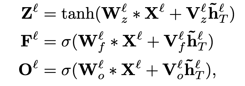
Next, we use extra kernel banks based on our pooling function (to be discussed in the next section), to get gated vectors like in LSTM:
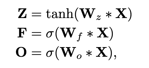
Here, * is the convolution operation; Z is the output discussed above (call it the ‘input gate’ output); F is the ‘forget gate’ output obtained using the extra kernel bank W_f; O is the ‘output gate’ output obtained using the extra kernel bank W_o.
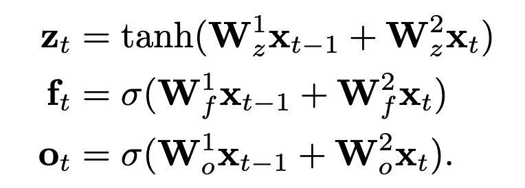
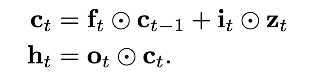
Fun fact: As discussed above, these convolutions are applied over the past ‘sequence_length - kernel_size + 1’ tokens only. So, if we take kernel_size = 2, we get LSTM-like equations:
The Pooling Component
Pooling, in general, is a parameter-less function that captures important features among the convoluted features. In case of images, usually, Max-Pooling and Average Pooling are used. However, we cannot simply take the average or the max between features in case of sequences. It needs to have some recurrence. Hence, the QRNN paper has proposed pooling functions inspired by the element-wise gated architecture in the traditional LSTM-cell. It is essentially a parameter-less function that will mix the hidden states across the timesteps.
The simplest option is “dynamic average pooling,” which uses just the forget gate (hence termed f-pooling):
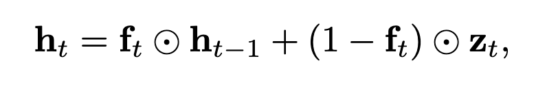
where ⊙ is element-wise matrix multiplication.
As you can see, it is more or less a ‘Moving Average’ of the output with the forget gate as the parameter.
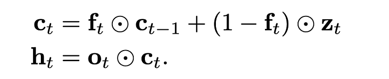
Another option is to use the forget gate as well as the output gate (hence, fo-pooling):
Or the pooling may additionally have a dedicated input gate (ifo-pooling):
Regularization
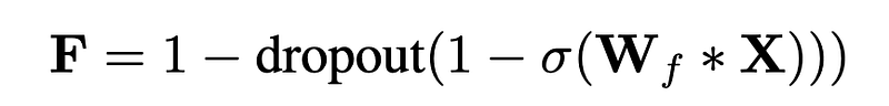
After examining various recurrent dropout schemes, QRNN uses an extension to a scheme called ‘zone out.’ It essentially selects a random subset of channels to dropout at each timestep, and for those channels, it simply copies the current channel value to the next time step without any modifications.
Conveniently, this is equivalent to stochastically setting a subset of the QRNN’s forget gate channels to 1, or applying dropout on 1−F.
Hence,
Ideas from DenseNet
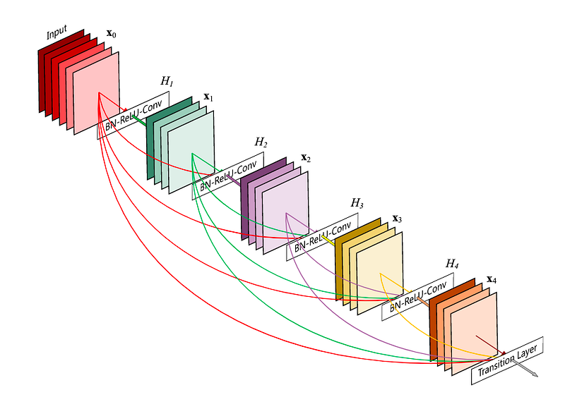
The DenseNet architecture suggests having skip-connections between each layer and every layer ahead of it, contrary to the convention of having skip-connections over subsequent layers. Thus, there would be L(L - 1) skip connections for a network with L layers. This helps gradient flow and convergence, but accounts for quadratic space.
seq2seq with QRNN
In a regular RNN-based seq2seq model, we simply initialize the decoder with the encoder’s last hidden state and then modify it further for the decoder sequence. Well, we cannot do this for the recurrent pooling layers as here, the encoder state wouldn’t be able to contribute much to the decoder’s hidden state. Hence, the authors have proposed a modified decoder architecture.
The last hidden state (hidden state of the last token) from the encoder is projected linearly (linear layer), and added (broadcasted as the encoder vector is smaller) to the convolution output of each timestep of the decoder layer before applying any activations:
~ means belonging to the encoder; V is the linear weight applied to the last encoder hidden state.
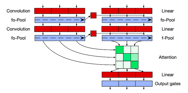
Attention
Attention is applied only to the last hidden state of the decoder.
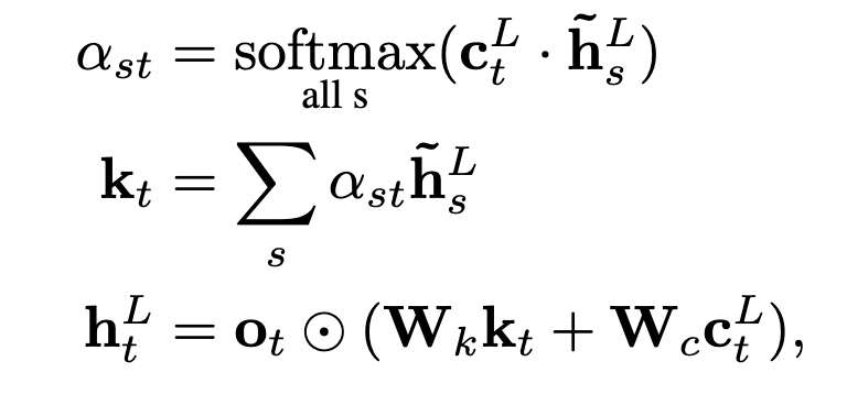
where s is the encoder’s sequence length, t is the decoder’s sequence length, L means the last layer.
First, the dot product of the un-gated last layer hidden states of the decoder is taken with the last layer encoder hidden states. This will result in a matrix of shape (t, s). Softmax is taken over s, and this score is used to obtain the attentional sum, k_t of shape (t, hidden_dim). k_t is then used alongside c_t to obtain the gated last layer hidden state for the decoder.
Results
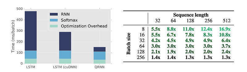
QRNN achieves comparable and, in some cases, slightly better results than the LSTM architectures with up to 17x faster computations.
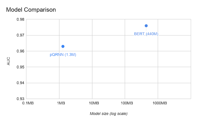
Recently a model, pQRNN, which is based on QRNN, has achieved comparable results to BERT on sequence classification with just 1.3M parameters (opposed to BERT, which is 440M parameters):
Conclusion
We discussed the novel QRNN architecture in depth. We saw how it adds recurrence to a convolution-based model and hence, speeds up sequence modeling. The speed and performance of QRNN definitely makes us reconsider transformers for some NLP tasks.


