Qrash Course II: From Q-Learning to Gradient Policy & Actor-Critic in 12 Minutes

Taking another step towards truly understanding the basics of Reinforcement Learning

Implementations of all algorithms discussed in this blogpost can be found on my GitHub page.

Read this blogpost even without being a Medium member using this Friends Link

The Qrash Course Series:

1. Part 1: Introduction to Reinforcement Learning and Q-Learning
2. Part 2: Policy Gradients and Actor-Critic

The previous — and first — Qrash Course post took us from knowing pretty much nothing about Reinforcement Learning all the way to fully understand one of the most fundamental algorithms of RL: Q Learning, as well as its Deep Learning version, Deep Q-Network. Let’s continue our journey and introduce two more algorithms: Gradient Policy and Actor-Critic. These two, along with DQN, are probably the most fundamental building-blocks of modern Deep Reinforcement Learning.

Why Isn’t Q-Learning Enough?

The first question we should probably ask ourselves is why should we advance from Q-Learning? Where does it fail or underperforms? Well, this algorithm does have a few pitfalls, and it’s important to understand them:

1. Poor performance over a large set of actions: Let’s assume an environment where the number of actions is large. Really large, say a few thousands, or even more. Exploring all possible actions using an ε-greedy strategy might take too long, and the algorithm can easily converge to a local maxima rather than the real best possible solution. Not so good.
2. Actions set must be finite: Let’s stretch the number of possible actions to its absolute limit: infinite. This is actually quite common — think of a self driving car, where the action is by how much to turn the wheel. This is a continuous range of numbers, and therefore infinite. It’s quite obvious why a Q-Learning algorithm cannot handle this case.
3. Poor exploration strategy: Let’s take an example — assume an environment where 10 different actions are possible, and a Q-Learning agent using an ε-greedy policy with ε = 0.1. Now let’s assume that action #1 is the one with the highest Q-Value at this given moment. This means that the agent has a chance of 91% to select action #1 (90% chance to select the greedy action + 1% of choosing this action at random), while all other actions have only a 1% chance of being selected. Now consider these Q-Values: Q(s, a¹) = 3.01, Q(s, a²) = 3.00, …, Q(s, a¹⁰) = 0.03. Even though the Q-Values of actions #1 and #2 are quite close, the chance of selecting #1 over #2 is significantly larger, as just explained. To make it even worse, the chance of selecting action #2 and #10 is exactly the same, even though action #2 is actually a hundred times (!!) better. Now combine this with the issue in section 1, and you can see why this might not be the best algorithm in this case.

How should we handle these situation? Let’s get to know our saviors!

Policy Gradients

A Q-Learning algorithms learns by trying to find each state’s action-value function — the Q-Value function. Its entire learning procedure is based on the idea of figuring out the quality of each possible action, and select according to this knowledge. So Q-Learning tries to have complete and unbiased knowledge of all possible moves — which is also its most major drawback, as this requires sufficient number of attempts of each possible state and action. Policy Gradient algorithm learns in a more robust way, by not trying to evaluate the value of each action — but by simply evaluate which action should it prefer.

Let me illustrate it better: each model eventually has some learned-parameters which it tries to optimize (these are usually the neural-network’s weights). Let’s denote these parameters as θ. In DQN, the learning cycle is:

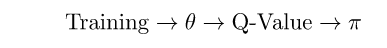
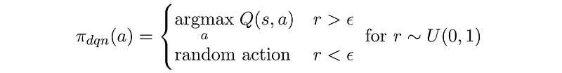
This means that the training procedure optimizes the learned parameters of the network, which is then used to compute Q-Values. We then use those Q-Values to decide on our policy π (where a policy is simply each action’s probability to be selected) — DQN’s ε-greedy policy depends on the predicted Q-Values, as it gives the highest probability to the action with the highest Q-Value:

The learning cycle of a Policy Gradient algorithm is shorter, skipping the Q-Value part:

This mean that the network will directly output the probability of selecting each action, skipping the extra calculation. This will allow this algorithm to be more robust.

We’re now left with one very important question — how do we optimize the network’s weights? In DQN it was straightforward: we know how to calculate Q-Values, so we can optimize the algorithm according to them. But what do we do now? Well, our main goal it to make sure to model gets better after each learning phase. Let’s try to write this as a very general update rule of the weights at each time step t as:

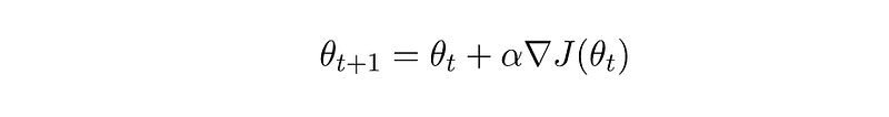
where we defined J as some performance measure, which we’ll get to in a second, and α is a learning rate. I’d like to take a minute to clarify the difference between a time-step t, which indicates steps taken in an episode, and s, which marks states of an episode. States are defined by the environment, for example — all possible boards of chess. Steps are defined by the agent, and mark the sequence of states it has been through. That means that step t=3 and t=7 might be the same state s, as some environments allow an agent to return to the exact same state multiple times. On the other hand, each step t happens once and only once in each episode. Steps are a chronological time sequence.

Let’s go back to our update rule, which we defined as dependent on the gradient of our new J parameter. While it might look familiar to the back-propagation phase of Neural Networks training, there’s a super-important difference here: in Gradient Policy we wish to increase performance, and therefore we wish to maximize the derivative of J, and not minimize it. This is known as gradient ascent — contrary to gradient descent performed in back-propagation. It’s actually quite the same logic, just the other way around.

Designing our first Gradient Policy algorithm

At this point it’s kind of obvious that how we define J will make all the difference, but it’s also entirely up to us to decide what is the right definition. Let’s try to find something simple — something that depends on the Q-Value (even though the algorithm never calculates it). Recall that a Q-Value Q(s,a) is a measure of all the rewards the agent shall receive till the end of the episode, starting from state s and after performing action a. The sum of all rewards seems to be quite a good performance measurement — after all, the agent’s sole purpose is to increase its overall collected rewards. So we can use as our performance measure the total accumulated rewards over an entire episode:

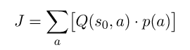
This is the sum of all Q-Values of the initial state s⁰, multiplied by probability to select each action. This exactly our expected overall reward of an entire episode. Now, this summation over all Q-Values of a certain state multiplied by their probabilities has a name: it’s called the state’s Value Function, and is denoted as V(s). A state’s Value Function is a measure of the expected reward from state s and till the end of the episode, without knowing which action will be chosen. So we basically defined the initial state’s Value Function as our performance measure: J = V(s⁰).

Now that we have J, we need to calculate its gradient. This involves some complex math, as J depends on the probability of action selection p(a), which is derived from the policy π — but π depends on J, since this is how we defined it. You can find the entire mathematical derivation in “Reinforcement Learning, An Introduction” by Sutton & Barto (2nd ed.), pages 325–327 (here’s a free online version). I’ll skip it here and write the down the solution:

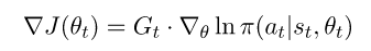
Where G_t is the total accumulated reward from step t till the end of the episode. This means the update rule for our θ is:

It might seems intimidating or bizarre to perform a logarithm of a policy — but it’s just another mathematical function we need to apply, nothing more.

Exploration and Exploitation

I’d like to emphasize again an important feature of the Policy Gradient algorithm — it learns the policy directly. This means the network’s input is the current state s and the output is the probability to select each action:

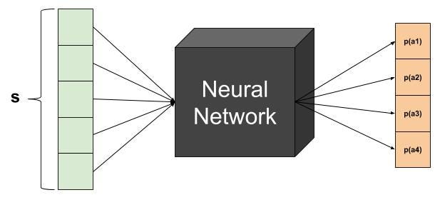
So how do we actually select an action? We simply perform a weighted-sampling over the action. This also solves our need of exploration — every action has a chance of being selected, but not equally, as the best action will be the most likely to be chosen.

Training

Unlike Q-Learning, the Policy Gradient algorithm is an on-policy algorithm — which means it learns only using state-action transitions made by the current active policy. Technically, this means there is not Experience Replay memory like in DQN. Once the model is trained, its θ parameters change, and therefore also it policy. This means that all experience collected before this training must be discarded, and cannot be used for training anymore. So every piece of data we collect for training is used once, and only once.

Gradient Policy in action

While the general idea is hopefully understood at this point, an example is always better. A very popular task to solve using Reinforcement Learning is the Cart-Pole problem: a cart, which can move either left or right, needs to make sure the pole which stands on it doesn’t fall. Here’s my solution to this challenge. Try to implement it yourself too.

Actor-Critic

Let’s take a minute to realize what we have developed so far: we now have an Agent that learns a policy without the need to learn the actual value of each action. The only thing it really needs is some performance metric, which it will try to maximize — and in our case we chose the total expected reward of an entire episode.

The benefits of this method is straightforward — there’s no need to visit and try each possible state-action pair, as the Agent develops some kind of a “gut-feeling” about what it should do. But this comes with a drawback due to the Agent’s absolute dependency in its performance metric. Let’s consider our case, where we chose the overall reward of an episode as the performance: consider an episode with a hundred steps taken. Each step yields a reward of +10, but step 47 yields a reward of -100. The performance measure we chose cannot distinguish this pitfall, as all it only knows the overall reward. This means our Agent might never try another action when it reaches step 47, as it doesn’t learn any state- and action-specific knowledge.

How can we tackle this? We would’ve liked to have an Agent that on one hand, learns a policy in a similar way to the Gradient Policy method, though on the other hand we understand the importance of state- and action-specific knowledge, like in the Q-Learning method. The solution? Combine the two together.

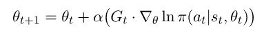
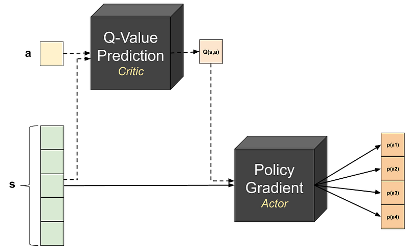
The combined method is known as Actor-Critic, and is made of two sub-Agents learning together: one learns the policy which should be acted by (and is therefore known as the Actor), and the other learns the Q-Value of each state and action (and is therefore known as the Critic). We then change our update rule of our θ to be:

Notice we simply replaced the total reward G with the Q-Value, but the Q-Value is now also a learned parameter — learned by the second sub-Agent. This yields a bit more complex architecture:

Note that just like Policy Gradients, Actor-Critics are also on-policy models — which again means that after each training, all previous training data is discarded.

And that’s it. You got it! You can try to implement an Actor-Critic yourself now, or check out my implementation solving the Acrobot challenge.

A2C, A3C and DDPG

We’re pretty much done here, but let’s take one more step forward and get to know some very useful optimizations to our Actor-Critic Agent.

A2C

Recall that we now use the Q-Value in our update rule in order to allow the Agent to have some state-action-specific knowledge. Now let me ask you a question: is Q(s,a)=100 a good Q-Value or not? The answer is — we don’t know. We don’t know because we don’t have information about the Q-Values of the other possible actions. If all other actions yield a Q-Value of 1, then 100 is really really good. But if all others yield 10,000 — then 100 is actually quite bad. This isn’t confusing only to you — but also to the model. It would have been helpful to know how good is a certain action compared to rest — or in other words, what is the advantage of taking a specific action. So we can replace the Q-Value in our Actor-Critic update rule with the Advantage of an action, which is defined as:

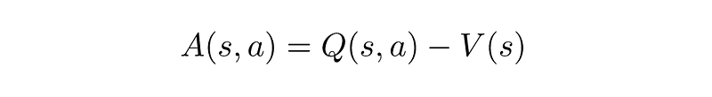
where V(s) is the state’s Value Function, which we’ve discussed before. Learning the advantage of an action is much easier— a positive A(s,a) is good, and a negative one is bad. This variation of the Actor-Critic model is known as the Advantage Actor-Critic, which is abbreviated to AAC, or more commonly: A2C (which is just a fancy way of writing that there are two As and a C).

You might notice that the A2C version seems to make learning a little more complex, as now the Agent needs to learn both Q(s,a) and V(s). But that’s actually not true. If a Q-Value is the reward received from state s and action a and then continuing till the end of the episode, we can write it like this:

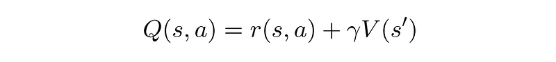
meaning — a Q-Value is actually the immediate reward r and the value of the next state, s’. This means we can write the Advantage as:

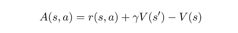
So we actually only need to learn the Value Function, and use it twice — for the state s and the next state s’. This little tweak actually makes the A2C easier to implement than the original Actor-Critic. You can check out my implementation of A2C on GitHub.

A3C

Why having only one Agent when we can have many? This is the core idea behind the A3C model, which stands for Asynchronous Advantage Actor-Critic. The idea is simple: have many different Agents, each playing in its own copy of the environment, but they all share the same policy and parameters. Each Agent update the shared policy on its own time (asynchronously of the other Agents), which makes the learning process faster and more robust.

DDPG

The DDPG (Deep Deterministic Policy Gradient) algorithm was designed with the problem of continuous action-space in mind. The training phase of an Actor-Critic model is very noisy, as it learns based on its own predictions. To tackle this, DDPG borrows some components from our beloved DQN: First, it uses an Experience Replay memory, which makes it an off-policy model. Second, it uses the same noise-reduction method of the Double DQN model — it uses two copies of both the Actor and the Critic, one copy is trained and the second is updated slowly, in the following way:

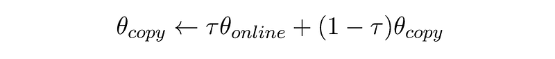
Here, the online network is the one trained, and τ << 1. See my implementation of DDPG for a more detailed explanation.

Final Words

In this tutorial, we’ve expanded our knowledge of the fundamental building-blocks of Reinforcement Learning, adding Gradient Policy and Actor-Critic to our arsenal of algorithms. Modern Reinforcement Learning is much more vast, but eventually it all relies on some similar ideas — which you now understand. Way to go!