Reinforcement Learning

Q-Learning Algorithm: How to Successfully Teach an Intelligent Agent to Play A Game

A detailed explanation of a Reinforcement Learning algorithm called Q-Learning with a step-by-step Python example

Intro

Reinforcement Learning (RL) is an exciting part of Machine Learning that helps us create intelligent agents capable of performing various tasks.

In this series of articles, I dive deeper into different RL techniques and show you how to apply them using Python code. This time I cover Q-Learning (Q stands for quality), one of the most straightforward RL approaches.

If you are unfamiliar with RL’s main ideas, feel free to refer to my introduction article: Reinforcement Learning (RL) — What Is It and How Does It Work?

Contents

• Where does Q-Learning sit within the broader Machine Learning (ML) universe
• Reinforcement Learning terminology
• How does Q-Learning work? - Difference between Policy-based and Value-based methods - Q-function and Q-table - Q-Learning algorithm - Q-Learning outputs
• Python example showing you how to train an agent to play a Frozen-Lake game

Q-Learning within the Machine Learning universe

The below chart is my attempt to categorise the most commonly used Machine Learning algorithms. Of course, it will never be perfect because some algorithms can fall into multiple categories. However, visualising the ML universe is extremely helpful, especially during a learning journey.

Q-Learning falls under the family of Reinforcement Learning algorithms and, more specifically, under the Value-based methods branch (more on that in the following sections).

The below chart is interactive, so please click👇 on different categories to explore and reveal more.

If you enjoy Data Science and Machine Learning, please subscribe to get an email with my new articles.

Reinforcement Learning terminology

Before we look at Q-Learning, here’s a quick recap of the fundamental elements of Reinforcement Learning:

• Agent — an “intelligent actor” that can interact with its environment, e.g. a player in a game.
• Environment — the “world” where that agent “lives” or operates.
• Action Space — a list or range of actions the agent can perform.
• State/Observation Space — a list or range of possible environment configurations. A state/observation provides information to the agent about its environment (e.g. its location).
• Reward — incentive (or disincentive) that we give to the agent when it performs desired (undesired) actions at various states. We can reduce future rewards relative to present rewards by using the discount factor {gamma(𝛾)}.
• Exploration/Exploitation {epsilon(𝜖)}— enables us to set how much time the agent should spend exploring the environment vs exploiting its existing knowledge about the environment.
• Episode — one complete cycle from the start position to the end position. E.g., in the context of a game, an episode would last from the moment your agent starts a new level until it dies or completes the level.
• Alpha(𝛼) — learning rate, which influences the learning speed and convergence towards the optimal policy.
• Policy(𝜋) —an agent’s strategy to pursue a goal.

How does Q-Learning work?

Difference between Policy-based and Value-based methods

Q-Learning falls into the category of Value-based methods, so let’s start by understanding the difference between Value-based and Policy-based methods.

• Policy-based methods — we train the agent directly on what action to take in which state. It is described by a policy function that can be either deterministic (gives the precise action for each state) or stochastic (provides a probability distribution over actions).
• Value-based methods — we train the agent indirectly by teaching it to identify which states (or state-action pairs) are more valuable so that it can be guided by value maximisation. It is described by a value function where the value of a state is the expected discounted return the agent can get if it starts in that state.

Regardless of which method we use to train our agent, finding the optimal policy function or the optimal value function equates to discovering the optimal policy(𝜋).

Q-function and Q-table

Since Q-Learning is a Value-based method, we must have a value function, which we will call a Q-function. Inside, it will have a Q-table containing every state-action pair.

Training a Q-function is simply finding the values associated with each state-action pair stored in a Q-table. Knowing these values enables the agent to choose the best action at each state.

In the later Python section, we will teach the agent to play a Frozen-Lake game, so let’s use the same game to demonstrate what a Q-table looks like.

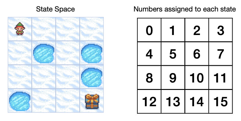
Our Frozen-Lake environment will be a 4x4 grid consisting of frozen squares and squares with holes, a total of 16 squares. Each square represents a possible state, which we can label by assigning numbers to them.

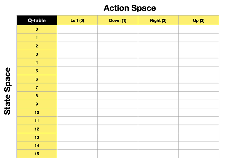
The action space will consist of 4 distinct actions that our agent can take: Left(0), Down(1), Right(2), Up(3).

Now we can form a Q-table with states as rows and actions as columns.

The game’s objective is for the agent to navigate from the start (square 0) to the finish (square 15 containing a present) without falling into a hole. So, training a Q-function will teach the agent how to avoid holes and find the fastest route to the goal.

Note, when we initialise the Q-table for the first time, it will have zeros in each cell as the agent will not know anything about its environment before it starts exploring it.

Q-Learning algorithm

Before we look at the actual Q-Learning algorithm, here are a couple more things to note:

• On-policy vs Off-policy: Q-Learning is an off-policy algorithm, which means that during training, we use different policies for the agent to act (acting policy) and to update the Q-function (updating policy). Meanwhile, On-policy means that the same policy is used for acting and updating. More on this in the Python section.
• Temporal Difference (TD) vs Monte Carlo: Q-Learning uses a TD approach, which means that during training, it updates the Q-function after each step. Meanwhile, the Monte Carlo approach is to wait until the end of the episode before making the update to the value function.

Now let’s take a look at the Q-Learning algorithm to see how it trains the Q-function (updates the Q-table):

• Q — Q-function
• 𝑆𝑡 — current state(observation)
• 𝐴𝑡 — current action
• 𝑅𝑡+1 — reward received following current action
• 𝑆𝑡+1 — next state(observation)
• 𝛼 (alpha) — learning rate parameter
• 𝛾 (gamma) — discount factor parameter
• 𝑚𝑎𝑥𝑎𝑄(𝑆𝑡+1,𝑎) — maximum value for the next state(observation) across the possible action space

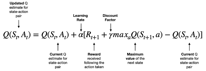
• The term on the left Q(𝑆𝑡,𝐴𝑡) is the new value for the specific state-action pair.
• The first term on the right-hand side, Q(𝑆𝑡,𝐴𝑡), is the current value for that same state-action pair.
• To modify the current value, we take the reward following the action taken by the agent 𝑅𝑡+1 add the maximum value we can get from the next state 𝛾𝑚𝑎𝑥𝑎𝑄(𝑆𝑡+1,𝑎) discounted by gamma, and subtract the current value Q(𝑆𝑡,𝐴𝑡).
• So, the terms in the square brackets can lead to either a positive, zero or negative value. Hence, the new Q value for that state-action pair will either increase, stay the same or reduce. Note that we also apply a learning rate to control the “size” of each update.

Since Q-Learning uses Temporal Difference (TD) approach, the algorithm will keep updating Q-table after each step until we reach a position where no more updates can be made, i.e., it has converged to an optimal solution.

Q-Learning outputs

Arriving at an optimal solution for a Q-function means that we have found the optimal policy(𝜋). Then, the agent can use this policy to successfully navigate its environment and achieve the highest cumulative rewards possible, depending on the starting state.

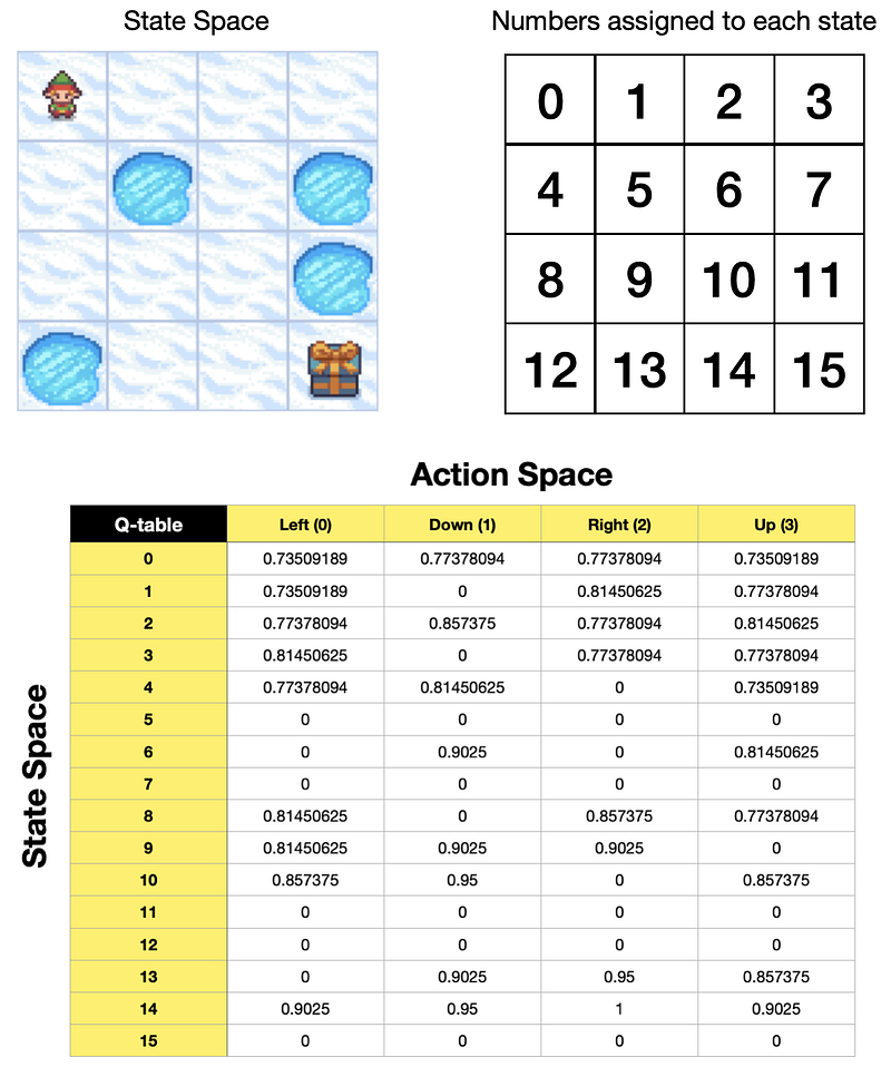
Here is the optimal Q-table for a Frozen-Lake game using 𝛾 (gamma) of 0.95 and the game’s default reward function:

• Reach goal(G): +1
• Reach hole(H): 0
• Reach frozen(F): 0

We will see how we arrive at this result in the Python section, but for now, let’s look at what it tells us.

If our agent was to use the policy described in the Q-table above, then:

• Starting from state 0, it is equally valuable to go either down or right. Based on the order of actions in our Q-table, the agent will go down to state 4.
• From state 4, the highest value action is to go down again, so it will do just that, reaching state 8.
• From state 8, the highest value action is to go right, taking the agent to state 9.
• From state 9, it is equally valuable to go down or right. But, again, since down comes first based on the order of actions in the Q-table, the agent goes down to state 13.
• From state 13, it will go right to state 14 and then right again to state 15, reaching the goal.

Here is a gif image of the agent following the above policy.

Python example showing you how to train an agent to play a Frozen-Lake game

Let’s now use Python to implement what we’ve just learned. We will use Open AI’s Gym Python library that contains various game environments, including Frozen-Lake.

Setup

We will need to get the following libraries:

• Open AI’s Gym library for the Frozen-Lake game environment
• Numpy for data manipulation
• Matplotlib and built-in IPython and time libraries for displaying how the agent navigates its environment

Let’s import the libraries:

import numpy as np
print('numpy: %s' % np.__version__) # print version

# Note need to 'pip install gym', and 'pip install gym[toy_text]' 
                                  # or 'pip install gym\[toy_text\]' if zsh does nor recongize the first command
import gym # for simulated environments
print('gym: %s' % gym.__version__) # print version

import matplotlib
import matplotlib.pyplot as plt # for displaying environment states
print('matplotlib: %s' % matplotlib.__version__) # print version

from IPython import display # for displaying environment states
import time # for slowing down rendering of states by adding small time delays

The above code prints package versions used in this example:

numpy: 1.23.3
gym: 0.26.0
matplotlib: 3.6.0

Next, we set up a Frozen-Lake environment:

# Setup environment
env = gym.make(id='FrozenLake-v1', # Choose one of the existing environments
               desc=None, # Used to specify custom map for frozen lake. E.g., desc=["SFFF", "FHFH", "FFFH", "HFFG"].
               map_name='4x4', # ID to use any of the preloaded maps. E.g., '4x4', '8x8'
               is_slippery=False, # True/False. If True will move in intended direction with probability of 1/3 else will move in either perpendicular direction with equal probability of 1/3 in both directions.
               max_episode_steps=None, # default=None, Maximum length of an episode (TimeLimit wrapper).
               autoreset=False, # default=None, Whether to automatically reset the environment after each episode (AutoResetWrapper).
               disable_env_checker=None, # default=None, If to run the env checker
               render_mode = 'rgb_array' # The set of supported modes varies per environment. (And some third-party environments may not support rendering at all.)
              )

Note that we use a non-slippery version of the game in this example. Meanwhile, the rendering options are as follows:

• None (default): no render is computed.
• human: render return None. The environment is continuously rendered in the current display or terminal, usually for human consumption.
• rgb_array: return frames representing the state of the environment. A frame is a numpy.ndarray with shape (x, y, 3), representing RGB values for an x-by-y pixel image.
• ansi: Return a list of strings (str) or StringIO.StringIO containing a terminal-style text representation for each time step. The text can include newlines and ANSI escape sequences (e.g. for colours).

Let’s check the environment description, state space and action space of the environment that we have set up above:

# Show environment description (map) as an array
print("Environment Array: ")
print(env.desc)

# Observation and action space 
state_obs_space = env.observation_space # Returns sate(observation) space of the environment.
action_space = env.action_space # Returns action space of the environment.
print("State(Observation) space:", state_obs_space)
print("Action space:", action_space)

Environment Array: 
[[b'S' b'F' b'F' b'F']
 [b'F' b'H' b'F' b'H']
 [b'F' b'F' b'F' b'H']
 [b'H' b'F' b'F' b'G']]

State(Observation) space: Discrete(16)
Action space: Discrete(4)

You can see that the environment matches the layout shown in the previous section. However, you can always specify your own map using the desc option within the gym.make(). Reminder: S = Start, F = Frozen, H = Hole, G = Goal.

Also, as expected, the state space contains 16 discrete states (4x4), and the action space has 4 discrete actions (0: LEFT, 1: DOWN, 2: RIGHT, 3: UP).

As a last check, before we do any training, we will let our agent loose around its environment (taking random actions at each step) and render it in the Jupyter Notebook.

# Reset environment to initial state
state, info = env.reset()

# Cycle through 20 random steps redering and displaying the agent inside the environment each time
for _ in range(20):
    
    # Render and display current state of the environment
    plt.imshow(env.render()) # render current state and pass to pyplot
    plt.axis('off')
    display.display(plt.gcf()) # get current figure and display
    display.clear_output(wait=True) # clear output before showing the next frame
    
    # Sample a random action from the entire action space
    random_action = env.action_space.sample()
    
    # Pass the random action into the step function
    state, reward, done, _, info = env.step(random_action)
        
    # Wait a little bit before the next frame
    time.sleep(0.2)
    
    # Reset environment when done=True, i.e., when the agent falls into a Hole (H) or reaches the Goal (G)
    if done:
        # Render and display current state of the environment
        plt.imshow(env.render()) # render current state and pass to pyplot
        plt.axis('off')
        display.display(plt.gcf()) # get current figure and display
        display.clear_output(wait=True) # clear output before showing the next frame
        # Reset environment
        state, info = env.reset()

# Close environment 
env.close()

Here is the output from the above code:

Training the Q-function to find the best policy

With the setup complete, let’s use Q-Learning to find the best policy(𝜋) for our agent to follow in this game.

We start by initialising a few parameters:

# Q-function parameters
alpha = 0.7   # learning rate
gamma = 0.95  # discount factor

# Training parameters
n_episodes = 10000  # number of episodes to use for training
n_max_steps = 100   # maximum number of steps per episode

# Exploration / Exploitation parameters
start_epsilon = 1.0  # start training by selecting purely random actions
min_epsilon = 0.05   # the lowest epsilon allowed to decay to
decay_rate = 0.001   # epsilon will gradually decay so we do less exploring and more exploiting as Q-function improves

Note that we will vary epsilon throughout training. We will start with epsilon=1, meaning that our agent’s actions will be all random at the beginning. However, we will decay epsilon with every episode, so our agent gradually moves from pure exploration to exploitation.

Next, let’s initialise the Q-table. As we’ve seen in the previous section, it will be a 16x4 table where 16 rows represent 16 states, and 4 columns represent 4 possible actions. We initialise the Q-table with all 0’s since we do not know how valuable each state is before we start the training.

# Initial Q-table
# Our Q-table is a matrix of state(observation) space x action space, i.e., 16 x 4
Qtable = np.zeros((env.observation_space.n, env.action_space.n))

# Show
Qtable

The above code displays the initialised Q-table:

array([[0., 0., 0., 0.],
       [0., 0., 0., 0.],
       [0., 0., 0., 0.],
       [0., 0., 0., 0.],
       [0., 0., 0., 0.],
       [0., 0., 0., 0.],
       [0., 0., 0., 0.],
       [0., 0., 0., 0.],
       [0., 0., 0., 0.],
       [0., 0., 0., 0.],
       [0., 0., 0., 0.],
       [0., 0., 0., 0.],
       [0., 0., 0., 0.],
       [0., 0., 0., 0.],
       [0., 0., 0., 0.],
       [0., 0., 0., 0.]])

Recall that Q-Learning is an off-policy algorithm. Hence, we will define one function for acting (epsilon_greedy) and another for updating the Q-table (update_Q). The updating policy uses a greedy approach, i.e. no exploration.

You should be able to spot that the update_Q function contains the Q-Learning algorithm equation analysed in the previous section.

# This is our acting policy (epsilon-greedy), for the agent to do exploration and exploitation during training
def epsilon_greedy(Qtable, state, epsilon):
    # Generate a random number and compare to epsilon, if lower then explore, itherwuse exploit
    randnum = np.random.uniform(0, 1)
    if randnum < epsilon:
        action = env.action_space.sample()    # explore
    else:
        action = np.argmax(Qtable[state, :])  # exploit
    return action


# This is our updating policy (greedy) 
# i.e., always select the action with the highest value for that state: np.max(Qtable[next_state])
def update_Q(Qtable, state, action, reward, next_state):
    # Q(S_t,A_t) = Q(S_t,A_t) + alpha [R_t+1 + gamma * max Q(S_t+1,a) - Q(S_t,A_t)]
    Qtable[state][action] = Qtable[state][action] + alpha * (reward + gamma * np.max(Qtable[next_state]) - Qtable[state][action])
    return Qtable


# This function (also greedy) will return the action from Qtable when we do evaluation
def eval_greedy(Qtable, state):
    action = np.argmax(Qtable[state, :])
    return action

Finally, let’s define our training function:

def train(n_episodes, n_max_steps, start_epsilon, min_epsilon, decay_rate, Qtable):
    for episode in range(n_episodes):
        
        # Reset the environment at the start of each episode
        state, info = env.reset()
        t = 0
        done = False
        
        # Calculate epsilon value based on decay rate
        epsilon = max(min_epsilon, (start_epsilon - min_epsilon)*np.exp(-decay_rate*episode))
        
        for t in range(n_max_steps):
            # Choose an action using previously defined epsilon greedy policy
            action = epsilon_greedy(Qtable, state, epsilon)
            
            # Perform the action in the environment, get reward and next state
            next_state, reward, done, _, info = env.step(action)
            
            # Update Q-table
            Qtable = update_Q(Qtable, state, action, reward, next_state)
            
            # Update current state 
            state = next_state
            
            # Finish the episode when done=True, i.e., reached the goal or fallen into a hole
            if done:
                break
                
    # Return final Q-table
    return Qtable

Now let’s call the training function and see the results:

# Train
Qtable = train(n_episodes, n_max_steps, start_epsilon, min_epsilon, decay_rate, Qtable)

# Show Q-table
Qtable

Following the training, we get the optimised Q-table, which matches the results we showed in the previous section. Now the agent can use it to always reach the Goal without falling into a Hole.

array([[0.73509189, 0.77378094, 0.77378094, 0.73509189],
       [0.73509189, 0.        , 0.81450625, 0.77378094],
       [0.77378094, 0.857375  , 0.77378094, 0.81450625],
       [0.81450625, 0.        , 0.77378094, 0.77378094],
       [0.77378094, 0.81450625, 0.        , 0.73509189],
       [0.        , 0.        , 0.        , 0.        ],
       [0.        , 0.9025    , 0.        , 0.81450625],
       [0.        , 0.        , 0.        , 0.        ],
       [0.81450625, 0.        , 0.857375  , 0.77378094],
       [0.81450625, 0.9025    , 0.9025    , 0.        ],
       [0.857375  , 0.95      , 0.        , 0.857375  ],
       [0.        , 0.        , 0.        , 0.        ],
       [0.        , 0.        , 0.        , 0.        ],
       [0.        , 0.9025    , 0.95      , 0.857375  ],
       [0.9025    , 0.95      , 1.        , 0.9025    ],
       [0.        , 0.        , 0.        , 0.        ]])

Evaluation

Let’s evaluate this policy by running a few simulations and checking if the agent always manages to get the maximum reward.

def evaluate_agent(n_max_steps, n_eval_episodes, Qtable):
    # Initialize an empty list to store rewards for each episode
    episode_rewards=[]
    
    # Evaluate for each episode
    for episode in range(n_eval_episodes):
        
        # Reset the environment at the start of each episode
        state, info = env.reset()
        t = 0
        done = False
        tot_episode_reward = 0
        
        for t in range(n_max_steps):
            
            # Use greedy policy to evaluate
            action = eval_greedy(Qtable, state)

            # Pass action into step function
            next_state, reward, done, _, info = env.step(action)

            # Sum episode rewards
            tot_episode_reward += reward

            # Update current state 
            state = next_state
            
            # Finish the episode when done=True, i.e., reached the goal or fallen into a hole
            if done:
                break
                
        episode_rewards.append(tot_episode_reward)
        
    mean_reward = np.mean(episode_rewards)
    std_reward = np.std(episode_rewards)

    return mean_reward, std_reward


# Call the above evaluation function and display the results:
n_eval_episodes=100 # evaluate over 100 episodes
mean_reward, std_reward = evaluate_agent(n_max_steps, n_eval_episodes, Qtable)
print(f"Mean Reward = {mean_reward:.2f} +/- {std_reward:.2f}")

The above code prints the following results:

Mean Reward = 1.00 +/- 0.00

As you can see, in every episode out of 100 episodes tested, the agent managed to get the maximum reward (1.00).

Let’s also evaluate it visually by making the agent follow the policy and render it on the screen:

# Cycle through 19 steps redering and displaying environment state each time
state, info = env.reset()
for _ in range(19):
    
    # Render and display current state of the environment
    plt.imshow(env.render()) # render current state and pass to pyplot
    plt.axis('off')
    display.display(plt.gcf()) # get current figure and display
    display.clear_output(wait=True) # clear output before showing the next frame
    
    # Use greedy policy to evaluate
    action = eval_greedy(Qtable, state)
    
    # Pass action into step function
    state, reward, done, _, info = env.step(action)

    # Wait a little bit before the next frame
    time.sleep(0.2)
    
    # Reset environment when done=True, i.e. when the agent falls into a Hole (H) or reaches the Goal (G)
    if done:
        # Render and display final state of the environment
        plt.imshow(env.render()) # render current state and pass to pyplot
        plt.axis('off')
        display.display(plt.gcf()) # get current figure and display
        display.clear_output(wait=True) # clear output before showing the next frame
        state, info = env.reset()

env.close()

The results are as expected, as we have seen in the previous section:

Final remarks

We have successfully employed Q-Learning to find the best policy for the agent to use in the Frozen-Lake game. I hope the game’s simple nature made it easy to understand how Q-Learning works.

Please don’t forget to subscribe, so you get to learn from my upcoming articles about other Reinforcement Learning algorithms and see how to apply them to different environments using Python!

You can find a complete Python code used in this article as a Jupyter Notebook on my GitHub repository.

Cheers! 🤓 Saul Dobilas