PyTorch Introduction — Building your First Linear Model

Learn how to build your first PyTorch model, by using the “magical” Linear layer

Regression Model — Image generated by AI

In my last blog post, we’ve learned how to work with PyTorch tensors, the most important object in the PyTorch library. Tensors are the backbone of deep learning models so naturally we can use them to fit simpler machine learning models to our datasets.

Although PyTorch is known for its Deep Learning capabilities, we are also able to fit simple linear models using the framework — and this is actually one of the best ways to get familiar with the torch API!

In this blog post, we’re going to continue with the PyTorch introduction series by checking how we can develop a simple linear regression using the torch library. In the process, we’ll learn about torch Optimizers, Weights and other parameters of our learning model, something that will be extremely useful for more complex architectures.

Let’s start!

Loading and Processing Data

For this blog post, we’ll use the song popularity dataset where we’ll want to predict the popularity of a certain song based on some song features. Let’s take a peek at the head of the dataset below:

songPopularity = pd.read_csv(‘./data/song_data.csv’)

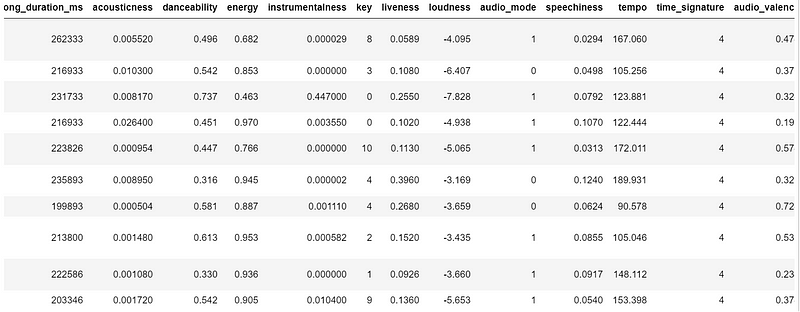
Song Popularity Feature Columns — Image by Author

Some of the features of this dataset include interesting metrics about each song, for example:

a level of song “energy”
a label encoding of the key (for example, A, B, C, D, etc.) of the song
Song loudness
Song tempo.

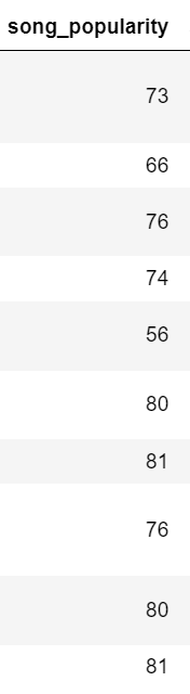
Our goal is to use these features to predict the song popularity, an index ranging from 0 to 100. In the examples we show above, we are aiming to predict the following song popularity:

Song Popularity Target Column— Image by Author

Instead of using sklearn, we are going to use PyTorch modules to predict this continuous variable. The good part of learning how to fit linear regressions in pytorch? The knowledge we’re going to gather can be applied with other complex models such as deep-layer neural networks!

Let’s start by preparing our dataset and subset the features and target first:

features = ['song_duration_ms', 
            'acousticness', 'danceability', 
            'energy', 'instrumentalness', 
            'key', 'liveness', 'loudness', 
            'audio_mode', 'speechiness', 
            'tempo', 'time_signature', 'audio_valence']

target = 'song_popularity'

songPopularityFeatures = songPopularity[features]
songPopularityTarget = songPopularity[target]

We’ll usetrain_test_split to divide the data into train and test. We’ll perform this transformation before transforming our data intotensors as sklearn ‘s method will automatically turn the data into pandas or numpy format:

X_train, X_test, y_train, y_test = train_test_split(songPopularityFeatures, songPopularityTarget, test_size = 0.2)

With X_train , X_test , y_train and y_test created, we can now transform our data into torch.tensor — doing that is easy by passing our data through the torch.Tensor function:

import torch

def dataframe_to_tensor(df):
    return torch.tensor(df.values, dtype=torch.float32)

# Transform DataFrames into PyTorch tensors using the function
X_train = dataframe_to_tensor(X_train)
X_test = dataframe_to_tensor(X_test)
y_train = dataframe_to_tensor(y_train)
y_test = dataframe_to_tensor(y_test)

Our objects are now intorch.Tensor format, the format expected by the nn.Module. Çet’s see X_train below:

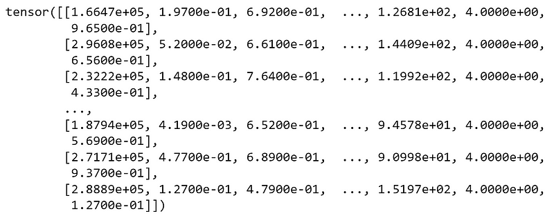
Cool — so we have our train and test data in tensorformat. We’re ready to create our first torch model, something that we will do next!

Building our Linear Model

We’ll train our model using a LinearRegressionModel classthat inherits from the nn.Module parent. The nn.Module class is Pytorch’s base class for all neural networks.

from torch import nn

class LinearRegressionModel(nn.Module):
    '''
    Torch Module class.
    Initializes weight randomly and gets trained via train method.
    '''
    def __init__(self, optimizer):
        super().__init__()
        self.optimizer = optimizer

        # Initialize Weights and Bias
        self.weights = nn.Parameter(
            torch.randn(1, 5, dtype=torch.float),
            requires_grad=True)

        self.bias = nn.Parameter(
            torch.randn(1, 5, dtype=torch.float),
            requires_grad=True
            )

In this class, we only need a single argument when creating an object — the optimizer. We’re doing this as we’ll want to test different optimizers during the training process. In the code above, let’s zoom in on the weight initialization right after # Initialize Weights and Bias:

self.weights = nn.Parameter(
 torch.randn(1, 13, dtype=torch.float),
 requires_grad=True)

self.bias = nn.Parameter(
            torch.randn(1, dtype=torch.float),
            requires_grad=True
            )

A linear regression is a very simple function consisting of the formula y = b0 + b1x1 + ... bnxn where:

y is equal to the target we want to predict
b0 is equal to the bias term.
b1, …, bn are equal to the weights of the model (how much each variable should weight in the final decision and if it contributes negatively or positively).
x1, …, xn are the values of the features.

The idea behind the nn.Parameter is to initialize b0 (the bias being initialized in self.bias) and the b1, … , bn (the weights being initialized in self.weights ). We are initializing 13 weights, given that we have 13 features in our training dataset.

As we’re dealing with a linear regression there’s only a single value for the bias, so we just initialize a single random scalar (check my first post if this name sounds alien to you!). Also, notice that we’re initializing these parameters randomly using torch.randn .

Now, our goal is to optimize these weights via backpropagation — for that we need to setup our linear layer, consisting of the regression formula:

def forward(self, x: torch.Tensor) -> torch.Tensor:
        return (self.weights * x + self.bias).sum(axis=1)

The trainModel method will help us perform backpropagation and weight adjustment:

    def trainModel(
            self,
            epochs: int,
            X_train: torch.Tensor,
            X_test: torch.Tensor,
            y_train: torch.Tensor,
            y_test: torch.Tensor,
            lr: float
            ):
        '''
        Trains linear model using pytorch.
        Evaluates the model against test set for every epoch.
        '''
        torch.manual_seed(42)
        # Create empty loss lists to track values
        self.train_loss_values = []
        self.test_loss_values = []

        loss_fn = nn.L1Loss()

        if self.optimizer == 'SGD':
            optimizer = torch.optim.SGD(
                params=self.parameters(),
                lr=lr
                )
        elif self.optimizer == 'Adam':
            optimizer = torch.optim.Adam(
                params=self.parameters(),
                lr=lr
                )

        for epoch in range(epochs):
            self.train()
            y_pred = self(X_train)
            loss = loss_fn(y_pred, y_train)
            optimizer.zero_grad()
            loss.backward()
            optimizer.step()

            # Set the model in evaluation mode
            self.eval()
            with torch.inference_mode():
                self.evaluate(X_test, y_test, epoch, loss_fn, loss)

In this method, we can choose between using between Stochastic Gradient Descent (SGD) or Adaptive Moment Estimation (Adam) optimizers. More importantly, let’s zoom in on what happens between each epoch (a pass on the entire dataset):

self.train()
y_pred = self(X_train)
loss = loss_fn(y_pred, y_train)
optimizer.zero_grad()
loss.backward()
optimizer.step()

This code is extremely important in the context of Neural Networks. It consists of the training process of a typical torch model:

We set the model in training mode using self.train()
Next, we pass the data through the model using self(X_train) — this will pass the data through the forward layer.
loss_fn calculates the loss on the training data. Our loss is torch.L1Loss that consists of the Mean Absolute Error.
optimizer.zero_grad() sets the gradients to zero (they accumulate every epoch, so we want them to start clean in every pass).
loss.backward() calculates the gradient for every weight with respect to the loss function. This is the step where our weights are optimized.
Finally, we update the model’s parameters using optimizer.step()

The final touch is revealing how our model will be evaluated using the evaluate method:

def evaluate(self, X_test, y_test, epoch_nb, loss_fn, train_loss):
        '''
        Evaluates current epoch performance on the test set.
        '''
        test_pred = self(X_test)
        test_loss = loss_fn(test_pred, y_test.type(torch.float))
        if epoch_nb % 10 == 0:
            self.train_loss_values.append(train_loss.detach().numpy())
            self.test_loss_values.append(test_loss.detach().numpy())
            print(f"Epoch: {epoch_nb} - MAE Train Loss: {train_loss} - MAE Test Loss: {test_loss} ")

This code performs a calculation of the loss in the test set. Also, we’ll use this method to print our loss in both train and test sets for every 10 epochs.

Having our model ready, let’s train it on our data and visualize the learning curves for train and test!

Fitting the Model

Let’s use the code we’ve built to train our model and see the training process — First, we’ll train a model using Adam optimizer and 0.001 learning rate for 500 epochs:

adam_model = LinearRegressionModel('Adam')

adam_model.trainModel(200, X_train, X_test, y_train, y_test, 0.001)

Here I’m training a model using the adam optimizer for 200 epochs. The overview of the train and test loss is shown next:

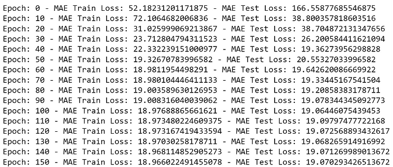
Train and Test evolution for the first 150 Epochs — Image by Author

We can also plot the training and test loss throughout the epochs:

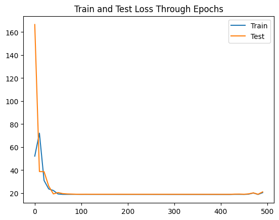
Our loss is still a bit high (on the last epoch, an MAE of around 21) as a linear regression may not be able to solve this problem.

Finally, let’s just fit a model with SGD :

sgd_model = LinearRegressionModel(‘SGD’)
sgd_model.trainModel(500, X_train, X_test, y_train, y_test, 0.001)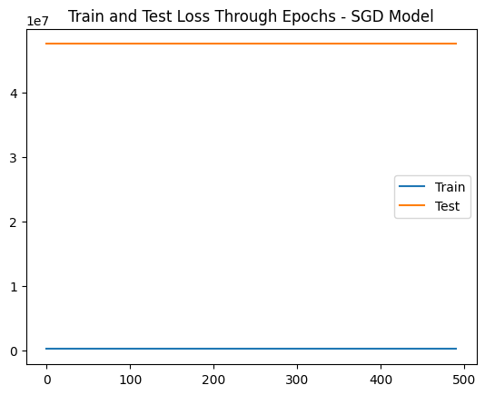

Train and Test Loss for SGD Model — Image by Author

Interesting — train and test loss do not improve! This happens because SGD is very sensitive to feature scaling and may have trouble calculating the gradient with features that have a different scale. As a challenge, try to scale the features and check the results with SGD . After scaling, you will also notice a stabler behavior on the Adam optimizer model!

Conclusion

Thank you for taking the time to read this post! In this blog post, we’ve checked how we can use torch to train a simple linear regression model. While PyTorch is famous for it’s deep learning (more layers and complex functions), learning simple models is a great way to play around the framework. Also, this is an excellent use case to get familiar with the concept of “loss” function and gradients.

We’ve also seen how the SGD and Adam optimizers work, particularly how sensitive they are to unscaled features.

Finally, I want you to retain the process that can be expanded to other types of models, functions and processes:

train() to set the model into training mode.
Pass the data through the model using torch.model
Using nn.L1Loss() for regression problems. Other loss functions are available here.
optimizer.zero_grad() sets the gradients to zero.
loss.backward() calculates the gradient for every weight with respect to the loss function.
Using optimizer.step() to update the weights of the model.

See you on the next PyTorch post! I also recommend that you visit PyTorch Zero to Mastery Course, an amazing free resource that inspired the methodology behind this post.

Feel free to join my newly created YouTube Channel — the Data Journey.

The dataset used in this blog post is available on the Kaggle Platform and was extracted using Spotify Official APP (https://www.kaggle.com/datasets/yasserh/song-popularity-dataset/data). The dataset is under license CC0: Public Domain