Python Pandas Library for Beginners: A Simplified Guide for Getting Started and Ditching Spreadsheets

Introduction

By the end of this guide you will be using pandas to create pivot tables just like you can in a spreadsheet, and you’ll have a foundation you can use to explore data using Python! I walk through the basics at first and get into more advanced concepts and examples later in the article. All the code can be found at the end of the article.

Why Pandas What is Pandas Installation Data Structures Reading Data Introduction to Exploring DataFrames Working with Data Selecting Data Common Operations and Functions Creating New Columns Sorting, Grouping and Pivoting Data

Why Pandas?

When I started in a six month program to learn data analytics, it comes at no surprise we started with spreadsheets in Excel. Excel and GoogleSheets are powerful tools, and I recommend everyone learn the basics like conditional formatting, simple aggregate functions, pivot tables, and visualizations. While spreadsheets are powerful tools, they start to break down or become difficult to use when handling large datasets. In the analytics course, once we started looking at datasets with millions of rows, we started learning Python and SQL.

A Programmer's Guide to Creating an Eclectic Bookshelf | Data Driven Investor

Every developer should have a bookshelf. The possible set of texts in his cabinet are myriad, but not every collection…

www.datadriveninvestor.com

When we started learning python, transitioning from Excel, pandas was one of the first libraries we explored. That is because one of its key data structures makes it easy to work with tabular data, which means data that has rows and columns like a spreadsheet. Since pandas 1.0 is officially out, I’m going back to basics and reminding myself of what I went through to build the foundation I have today.

pandas documentation - pandas 1.0.1 documentation

API reference The reference guide contains a detailed description of the pandas API. The reference describes how the…

pandas.pydata.org

What is pandas?

Thanks to the founding developer, Wes McKinney, the pandas library is open source and has a solid community backing it. It is used in data analysis and data science as a data manipulatin tool… Safe to say it handles a lot of data. Before Wes left the hedgefund he worked at while developing pandas, he convinced the company to allow him to open source the library. What a good move!

Under the hood, pandas uses Cython or C, making it quite powerful and optimized for performance. Reading more and more about Python, one of the complaints that comes up is that it is slow in comparison to compiled code like C. Cython tries to bridge the gap by combining the power of Python and C. It is designed to make it easy to write C extensions for Python.

Installation and Dependencies

Installing pandas is simple. The documentation recommends using pip or conda to install the pandas package. When importing pandas, it is common to give it an alias of pd.

pip install pandas

OR

conda install pandas

import pandas as pd

Data Structures

Pandas has two data structures:

Although I will focus mostly on manipulating DataFrames, it is important to understand what a Series is. A pandas Series is one-dimensional. It is an array that can hold any data type and it has a labeled axis, referred to as the index. Although similar, a Series has differences from a numpy array. Refer to the documentation to learn more about Pandas series.

import pandas as pd
example_series = pd.Series(data, index = your_index)

A pandas DataFrame stores data in a tabular format with integrated indexing. That means each column has a column name and each row has a row index. All of the examples will be using pandas DataFrames.

import pandas as pd
example_DataFrame = pd.DataFrame(data, index)

Reading Data

The pandas I/O API simplifies opening and writing to files. There are reader functions that typically return pandas objects like dataframes. There are writer functions, which are object methods, used to export the data out of pandas. In this example, I’ll use the reader function, pandas.read_csv() to open a .csv file. The file can be found on kaggle.

Comma Separated Values files, or csv for short, is a common file type when dealing with data since it easily transfers into a tabular form. They contain data like this:

column1,column2,column3 ,1,2,3 ,2,3,4 ,…

#import dependencies
import pandas as pd

#set the file path
filepath = r'Data\beef-jerky\jerky.csv'

Using read_csv to open the csv file into a pandas DataFrame

#open the csv data into a dataframe named df
df = pd.read_csv(filepath)

Now that the data is in a DataFrame object, it’s time to explore the data!

Introduction to Exploring DataFrames

Here are a the basics for exploring the data in a DataFrame:

Display the columns using .columns
Display the index using .index
Display the first 5 rows using .head()
Display the last 5 rows using .tail()
Display summary statistics using .describe()
Display the datatypes using .info()

Note that .head() and .tail() allow n to be passed into it:

#Example of n values
dataframe.head(1) #returns top 1 row
datafrare.tail(10) #returns last 10 rows

#display the columns
df.columns

#display the index
df.index

#Display the first 5 rows using .head()
df.head()

#Display the last 5 rows using .tail()
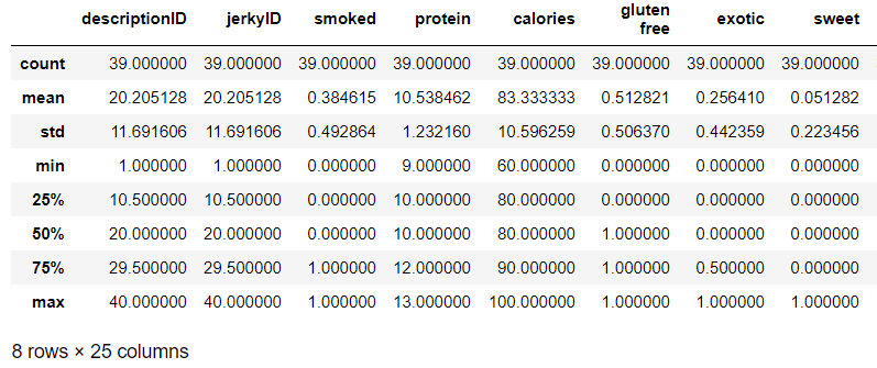
df.tail()

#generate statistics 
df.describe()

Using DataFrame.describe() returns some basic descriptive statistics about the numerical columns in the dataframe.

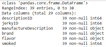
#display the columns and data types
df.info()

Using DataFrame.info() returns the data types for each column, as well as general information about the size and shape of the dataframe.

Working with Data

It is possible to select one or more columns and perform operations on them. For example, I might want to create a dataframe using only numeric columns, dropping any column that contains text. I’ll show four examples:

Select one column from a dataframe(two differeny syntax examples)
Select two columns from a dataframe
Selecting the unique values from a column using .unique()
Selecting the count of unique values from a column using .nunique()

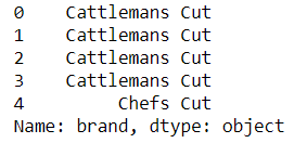
#only select the brand column
df['brand'].head()

OR

df.head()['brand']

I prefer using the first way since that is how I learned, but regardless of how it is written, both will return the same result.

Select multiple columns from the dataframe using a double set of brackets like this: DataFrame[[]]

#selcet the brand and flavor column. Notice the double bracket [[]]
df[['brand', 'flavor']].head()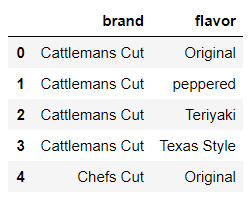

Use DataFrame[‘column’].unique() to return an array of the unique values in a column. This is extremely useful when working with categorical data!

Use DataFrame[‘column’].nunique() to return a distinct count of unique values in the column.

#return unique values
print(df['brand'].unique())
print(df['brand'].nunique())

print(df[‘brand’].unique()) AND print(df[‘brand’].nunique())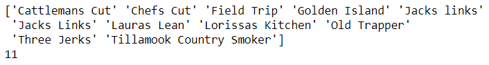

If using a time series, the feature DataFrame[‘column’].pct_change() comes in handy. It computes the percentage change from the previous row by default. Refer to documentation for a complete explanation.

Selecting Data

There are three basic ways to select data in pandas. Data can be selected in slices using brackets [ ], or using the .loc[ ] attribute. It can also be selected by integer using .iloc[ ]. I recommend reviewing the documentation for more advanced data selection techniques. I’ll show these examples:

* Select rows 5 and 6 using a slice * Select Original flavor using .loc[ ] * Select using iloc

#slicing the dataframe
df[['brand','flavor']][5:7]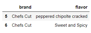

Be careful not to overuse this method when you need to manipulate data. I’ll discuss copying data later on. Refer to the documentation for a complete breakdown of the differences between slicing and using .loc methods.

Also, notice rows 5 and 6 return. That is because the index of a dataframe starts at 0 and the slice is exclusive of the last value, not inclusive.

#return the rows with a value Original in column flavor
df[['brand','flavor']].loc[df['flavor'] == 'Original']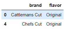

Use DataFrame.iloc[] to pass index values instead of columns. For example, this will return the two records for Original flavor:

#return the rows with a value Original in column flavor
df[['brand','flavor']].iloc[[0,4]]

Common Operations and Functions

Pandas makes it easy to generate some descriptive statistics using operations like mean and count. A quick reference of functions can be found in the documentation

Use .count() to find the number of rows
Use .mean() to find the mean sodium value
Use .median() to find the median sodium value
Use .mode() to find the mode sodium value
Use .min() to find the minimum sodium value
Use .max() to find the maximum sodium value

#Use .Count() to find the number of rows
df[['brand', 'flavor']].count()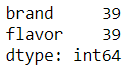

#Use .mean() to find the mean sodium value
df['sodium'].mean()
#438.3333333333333

# Use .median() to find the median sodium value
df['sodium'].median()
#470.0

# Use .mode() to find the mode sodium value
df['sodium'].mode()
#520

# Use .min() to find the minimum sodium value
df['sodium'].min()
#140

# Use .max() to find the maximum sodium value
df['sodium'].max()
#650

Creating New Columns

Adding a new column is easy. This is the basic syntax I use:

DataFrame[‘column name’] = something

Before modifying the dataframe, I think it is a good idea to copy it. That way I can always refer to the original if I make a mistake. Create a copy using DataFrame.copy()

Create a new copy of the dataframe named df_copy.
Create a new column and set each row to a value of 1.
Display the top 3 rows for brand, flavor, and the new column.

#make a copy
df_copy = df.copy()

#add a new column
df_copy['My_New_Column'] = 1

#display the new column
df_copy[['brand','flavor','My_New_Column']].head(3)

df_copy[[‘brand’,’flavor’,’My_New_Column’]].head(3)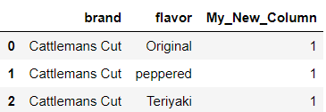

Adding new columns can be very useful. For example, say I wanted to compare the sodium to the mean value. I can add the mean as a column.

#create a new column displaying the mean value of sodium
df_copy['sodium_mean'] = df['sodium'].mean()
df_copy[['brand','flavor','sodium','sodium_mean']].head(3)

df_copy[[‘brand’,’flavor’,’sodium’,’sodium_mean’]].head(3)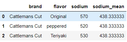

More Advanced Columns

Here are a couple advanced examples to show off different ways to add columns or engineer features.

Create an Above_average_cost column that outputs a 1 if the cost is greater than the average. Else 0.
Create a word_count column that outputs the number of words in the manufactureDescription column.

There are probably multiple ways to approach the problems, but I’ll show you two. First, I will show how it can be done using a simple for loop.

#use a for loop to create a new column
average_calories = df_copy['calories'].mean()

above_average = []

for calories in df_copy['calories']:
    if calories > average_calories:
        above_average.append(1)
    else:
        above_average.append(0)

df_copy['above_average_calories'] = above_average

The for loop is not optimal; look at all that code! I can imagine using a for loop if the readability is of utmost important, but most often I will go the pythonic route and try to use a list comprehension.

#Use list comprehensions to create new columns

#Create a new column that outputs a 1 if the cost is greater than #the average. Else 0
df_copy['above_average_calories'] = [1  if n > average_calories else 0 for n in df_copy['calories']]

#Create a word_count column that outputs the number of words in the #manufactureDescription
df_copy['word_count'] = [len(str(words).split(" ")) for words in df_copy['manufactureDescription']]

#Display the top 3 rows
df_copy[['brand','flavor','above_average_calories','word_count']].head(3)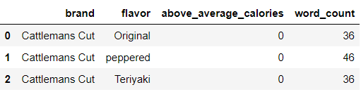

Another way to create a word count column is to use pandas DataFrame[‘column’].apply(). It might feel a little tricky at first, but apply lets me apply a function along the axis of a dataframe. What that means is I can apply a function to each column or row. In the example below, I use .apply() to apply a lambda function to each column (axis = 0 by default) of the dataframe.

#Create a new column that outputs the number of words in the manufactureDescription
df_copy['word_count']= df_copy['manufactureDescription'].apply(lambda x: len(str(x).split(" ")))

Sorting, Grouping and Pivoting Data

The concepts and science behind pivoting, grouping and sorting data can be hard to explain, and honestly an article all its own. While sorting is fairly straight forward(ascending and descending), grouping is typically used for splitting data, applying a function to grouped data, or combining results into a data structure. Here are a couple examples of how to apply .sort_values() and .groupby().

Sort the data by calories descending
Calculate the mean protein and calories grouped by brand.

#sort the data 
df_copy[['brand','protein', 'calories','flavor']].sort_values('calories', ascending = False)

#group by brand and calc mean
df_copy[['brand','protein', 'calories','gluten free']].groupby('brand').mean()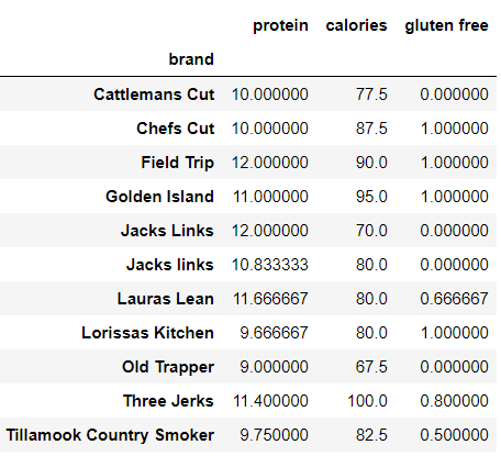

For the pivot table example, import numpy to use aggregate functions. Pivot tables can also be created in a few lines of code! Use pandas.pivot_table() to create a spreadsheet-like pivot table.

import numpy as np
pd.pivot_table(df_copy, index = ['brand'], values = ['calories'], aggfunc = np.mean)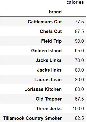

Wrapping Up

Congratulations on reaching the end of the beginner guide to pandas. I covered tons of concepts that will build a foundation from which anyone can explore a data set. Loading a file into a dataframe is simple, and pandas makes it easy to generate statistics and engineer new columns. Here is the complete set of examples!

#import dependencies
import pandas as pd
#set the file path
filepath = r'Data\beef-jerky\jerky.csv'

#open the csv data into a dataframe named df
df = pd.read_csv(filepath)

#Example of n values
dataframe.head(1) #returns top 1 row
datafrare.tail(10) #returns last 10 rows
#display the columns
df.columns
#display the index
df.index
#Display the first 5 rows using .head()
df.head()
#Display the last 5 rows using .tail()
df.tail()
#generate statistics 
df.describe()

#display the columns and data types
df.info()

#only select the brand column
df['brand'].head()
OR
df.head()['brand']

#selcet the brand and flavor column. Notice the double bracket [[]]
df[['brand', 'flavor']].head()

#return unique values
print(df['brand'].unique())
print(df['brand'].nunique())

#slicing the dataframe
df[['brand','flavor']][5:7]

#return the rows with a value Original in column flavor
df[['brand','flavor']].loc[df['flavor'] == 'Original']

#return the rows with a value Original in column flavor
df[['brand','flavor']].iloc[[0,4]]

#Use .Count() to find the number of rows
df[['brand', 'flavor']].count()

#Use .mean() to find the mean sodium value
df['sodium'].mean()
#438.3333333333333
# Use .median() to find the median sodium value
df['sodium'].median()
#470.0
# Use .mode() to find the mode sodium value
df['sodium'].mode()
#520
# Use .min() to find the minimum sodium value
df['sodium'].min()
#140
# Use .max() to find the maximum sodium value
df['sodium'].max()
#650

#make a copy
df_copy = df.copy()
#add a new column
df_copy['My_New_Column'] = 1
#display the new column
df_copy[['brand','flavor','My_New_Column']].head(3)

#create a new column displaying the mean value of sodium
df_copy['sodium_mean'] = df['sodium'].mean()
df_copy[['brand','flavor','sodium','sodium_mean']].head(3)

#use a for loop to create a new column
average_calories = df_copy['calories'].mean()
above_average = []
for calories in df_copy['calories']:
    if calories > average_calories:
        above_average.append(1)
    else:
        above_average.append(0)
df_copy['above_average_calories'] = above_average

#Use list comprehensions to create new columns
#Create a new column that outputs a 1 if the cost is greater than #the average. Else 0
df_copy['above_average_calories'] = [1  if n > average_calories else 0 for n in df_copy['calories']]
#Create a word_count column that outputs the number of words in the #manufactureDescription
df_copy['word_count'] = [len(str(words).split(" ")) for words in df_copy['manufactureDescription']]
#Display the top 3 rows
df_copy[['brand','flavor','above_average_calories','word_count']].head(3)

#Create a new column that outputs the number of words in the manufactureDescription
df_copy['word_count']= df_copy['manufactureDescription'].apply(lambda x: len(str(x).split(" ")))

#sort the data 
df_copy[['brand','protein', 'calories','flavor']].sort_values('calories', ascending = False)
#group by brand and calc mean
df_copy[['brand','protein', 'calories','gluten free']].groupby('brand').mean()

import numpy as np
pd.pivot_table(df_copy, index = ['brand'], values = ['calories'], aggfunc = np.mean)

Thank You!

If you enjoyed this, follow me on Medium for more
Get FULL ACCESS and help support my content by subscribing
Let’s connect on LinkedIn
Analyze Data using Python? Check out my website

— Eric Kleppen

Check out my other tutorials to see more advanced uses of pandas:

Dashboards in Python for Beginners and Everyone Else using Dash

Build a basic and advanced dashboard with this beginner tutorial on Dash in Python

medium.com

My Trick to Learning List Comprehensions in Python

What triggered my Eureka moment when working with List Comprehensions in Python

towardsdatascience.com

Web Scraping Board Game Descriptions with Python

How I scraped board game descriptions from the web.

towardsdatascience.com