Python for Geosciences: Working with Satellite Images (step by step)

First post in a series that will teach non-programmers how to use Python to handle and analyze geospatial data.

Update

For information about the course Introduction to Python for Scientists (available on YouTube) and other articles like this, please visit my website cordmaur.carrd.co.

Introduction

This is the first in a series of stories I intend to publish on how to use the Python programming language to work with geospatial data. After a few years working in the field, I notice that there are many professionals from geosciences and related areas who are not programmers but need, to some extent, use a programming language to perform analysis, math calculations or simply automate a workflow. Frequently, those professionals struggle to achieve this. Without proper knowledge, they end up developing complex codes without following best practices that are prone to errors and that are not efficient to handle the amount of data there is in geospatial field. At another extreme, we notice IT professionals who have mastered the concepts of programming but do not have the knowledge to work correctly with geospatial data. This series aims to fill precisely this gap.

Besides that, if you are like me and don’t have an IT background, some fundamental concepts for a good coding such as classes inheritance, operator overload, among others, are usually explained abstractly, or with examples that don’t make much sense in real life, causing disinterest making it difficult to be understood.

So, the main idea is to present basic to advanced Python concepts by examples extracted from Geosciences and Environmental thematic areas where we will manipulate geospatial data, being them matricial or vectorial. Contrary to most tutorials available online, we should follow a top-down approach, where we will first learn how to execute some important tasks and afterwards, go deeper into the necessary concepts. All necessary code to follow up the tutorial will be made available through Jupyter Notebooks (explained later).

If you are already familiarized with all these concepts, you can check my other posts on Machine and Deep learning for spatial data in my medium profile (https://cordmaur.medium.com/).

Step 1- Installation

Python Installation

As we are assuming that readers are not very familiar with programming, we chose to install Python in Windows environment, through the graphical interface, without worrying about the command line (at least at that moment, because as as we move forward, we will also use the command line for installing packages, downloading images, etc.). For some more advanced work, such as processing multiple geospatial images on a high-performance remote server, it will normally be necessary to use Python on Linux, but everything done on Windows will serve as the basis for future migration.

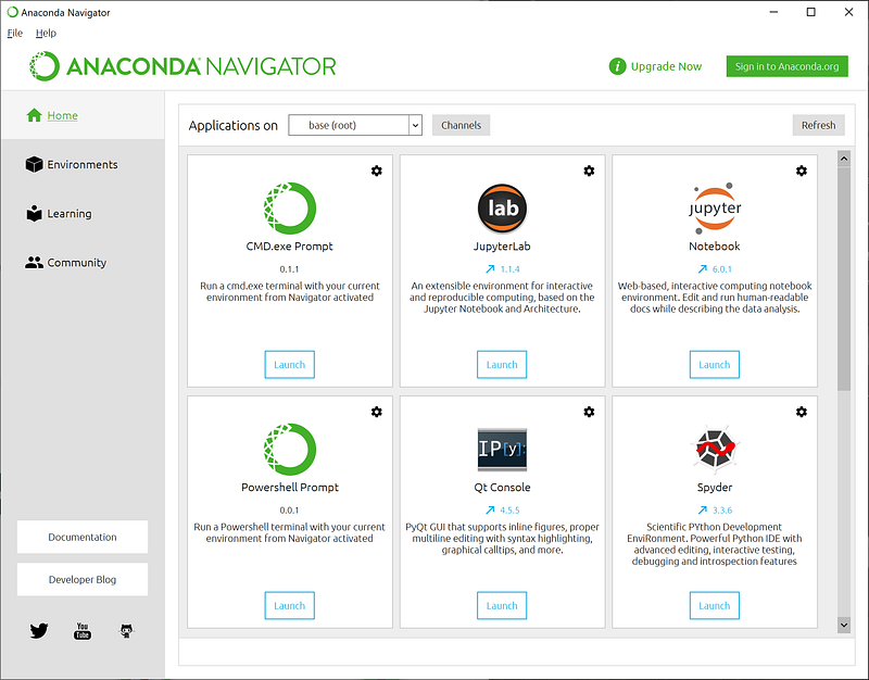
On Windows, the easiest way to have a Python environment ready to use is by installing the Anaconda package manager, available at: https://www.anaconda.com/products/individual

The installation follows the normal Windows workflow, through wizards. Once installed, Anaconda Navigator will be available to run.

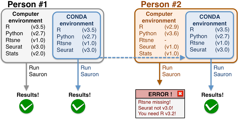
Figure 1: Anaconda Navigator initial screen. Image by author.

Before we start with our example, let’s create a specific environment for our code. Environments con be considered repositories in which Python packages are installed to in order to avoid conflicts between packages and versions. For example, if you have code developed using a NumPy 1.18 package and this code does not work with the current version which is 1.20, you can (and should) create specific environments for each version, as shown in Figure 2.

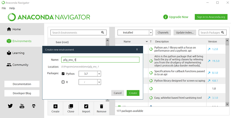
Figure 2: Anaconda environments example. Credit: https://nbisweden.github.io/workshop_omics_integration/conda_instructions.html

Conda comes initially with a standard environment called base(root). Before installing our packages we will create a new environment, by clicking on Environments tab on the left and the Create button below the list of environments. To this new environment, we can give a name “pfg_env_1” and select Python 3.7 as the main package (Figure 3).

Figure 3: Environment creation using Anaconda Navigator on Windows. Image by author.

To write and execute our code we will use Jupyter Lab, which is an evolution of Jupyter Notebook, with some additional functionalities. With the new environment selected, we should go back to Homeand click Install, just below the Jupyter Lab icon.

Packages Installation

Back to the Environments tab, we should click on the environment that we have just created to display the list of installed packages on the right window. The standard installation comes with several packages, but for our first example it will be necessary to install additional ones. Once again, we will use Anaconda’s graphical interface to search for and to install the necessary packages. Below is the list of packages that we need to install and the link to the original documentation for each one for future reference (we don’t need to worry about them at the moment).

NumPy (https://numpy.org/)
Matplotlib (https://matplotlib.org/)
Rasterio (https://rasterio.readthedocs.io/en/latest/)

To install a new package, it is necessary to search for the desired package name using the search bar (don’t forget to select All from the dropdown box), select the package from the list and click Apply.

Obs: As the packages work with dependencies, depending on the package to be installed it will install all the necessary packages that don’t exist yet in the current environment.

Figure 4 shows the procedure for installing Rasterio and the detail that NumPy is automatically installed as it is one of the non-existent dependencies.

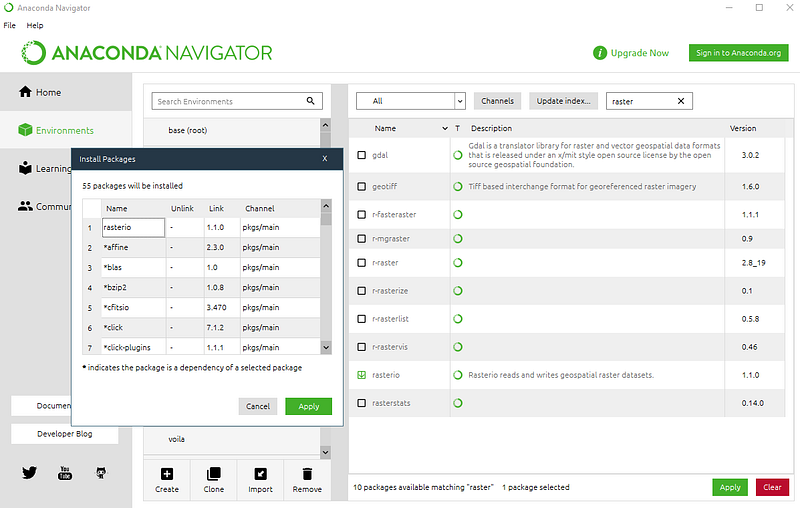
Figure 4: Package’s installation using Anaconda Navigator. Image by author.

We should repeat the same operation for Matplotlib (which we will be using for visualization) and then we are ready to proceed.

Starting Jupyter Lab

As already mentioned, Jupyter Lab is the environment that we will use to develop all of our work in Python. Jupyter Lab is an interactive web interface for code development, which follows the concept known as REPL (Read — Evaluate — Print — Loop), that is widely used by data scientists. The great advantage of using a REPL environment is that we can develop our code in a gradual manner, executing command by command and checking its results. Additionally, we can keep explanatory text together with the code that we are going to develop and also view the results, all in the same environment without need to alternate between the command line and other applications, such as image viewer or others.

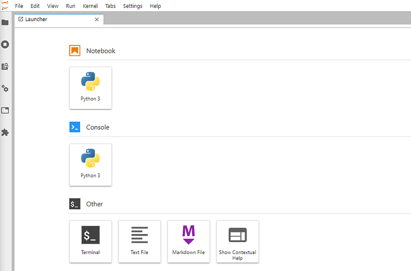
To start Jupyter Lab, it is necessary to go back to the Home tab and click on the Launch button below the corresponding icon. A new tab should open in the default system’s browser. After that, if you now have the screen as in Figure 5 congratulations, you have installed Python correctly.

Figura 5: Jupyter Lab initial screen. Image by author.

Step 2- Using the Jupyter Lab

Before moving on to our goal itself, let’s take a few moments just to learn the basics of Jupyter Lab. Other Python concepts like data types, working with lists, and many more will be introduced later, as we advance in the tasks. At this point we’ll look at just the very basics so we can proceed.

Initially we will click on the Notebook / Python 3 button to open a new notebook. Notebooks are initially created with the name UntitledX.ipynb, which can be changed later. Note that there are two types of cells in a notebook: Markdown and the code cells. Markdown cells are used to store headings, comments or any other static texts, that don’t need to be executed by the Python interpreter. The code cells contain information that will be effectively processed by Python to perform the requested calculation.

O primeiro botão à esquerda (FileBrowser) mostra a árvore de diretório e arquivos do nosso usuário. Como exemplo, vamos digitar inicialmente alguns comandos (o notebook 1, abaixo, possui diversos comandos para você poder executar e se ambientar) para vermos os resultados. Digite sempre os comandos Shift + Enter após finalizar o código de uma célula para executar os comandos e mostrar os resultados.

The first button on the left (FileBrowser) shows our user’s directory tree and files. As an example, let’s first type in some commands (Notebook 1, below, has several commands for you to execute and get used to the IDE) to see the results. Always type the commands Shift + Enter after finalizing the code of a cell to execute the commands and show the results.

Passo 3- Download Landsat 8 Imagery

Now that we have Python running and we already know how to execute simple commands, let’s get a satellite image that we want to open. To get started, we will use images from the Landsat 8 satellite, which are available for download on the USGS website (EarthExplorer). The site requires login with a free account. Figure 6, below, shows the step by step to download an image of the Manaus region (the capital of the Amazon State, Brazil) using the EarthExplorer.

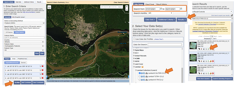
Figure 6: Downloading a Landsat 8 image from the USGS’s Earth Explorer site. Image by author.

Initially we browse the interactive map, zoom in on the region of interest and click on Use Map. Then we select the period of interest in my case from 1/1/2020 to 2/1/2021 for images with cloud cover between 0 and 20%, in order to avoid images with many clouds. Then we click on Data Sets to select the data collection we want (in this case the Landsat 8 Level 2A images, which means that these images have already undergone a first atmospheric correction, among others treatments) and finally we click on Results so that the system shows a list of images found according to the selected filters. In my example, I selected the image LC08_L2SP_231062_20201026_20201106_02_T1 and unzipped the content in a directory called “d:/Images/Landsat/”. The following files must be contained within the image directory:

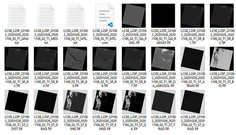
Figure 7: Landsat 8 image’s contents. Image by author.

Files ending with _SR_B? .Tif represent the atmospherically corrected surface reflectance for each of the bands of the OLI sensor (Operational Land Imager). The wavelengths of each band, as well as other technical information about the sensor, can be found on the page of the USGS itself (here).

Step 4- Opening a GeoTiff image

I mentioned GeoTiff in the section title because, at first, we will open only one “band” and not an entire image with the various bands, metadata, etc. To do this, we will use the Rasterio package that was already installed in Step 1. Initially we need to understand what a raster image represents in practice and what is the difference of a geospatial one.

Raster Image

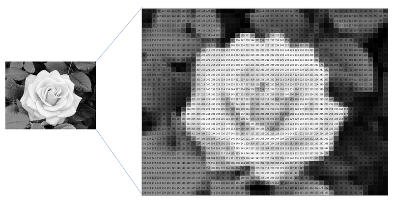
A raster image is one that can be represented by an array of values with n lines and m columns, where each value represents the intensity or “brightness” of that pixel. Figure 8 shows a grayscale image of a flower (in this case, only one “channel” or band) and the corresponding values for each pixel.

In addition, a geospatial raster image also has metadata to inform the location on the Earth’s surface where each of the values occurs. To solve this, an affine transformation (more on that can be found on Wikipedia) is additionally used, responsible for indicating the location of the matrix in an arbitrary space, and a coordinate reference system (CRS), which converts that space into a terrestrial location.

Loading the GeoTiff

The data types originally supported by Python are quite limited so, in order to manipulate more complex data (such as a Satellite Image) we usually rely on modules developed by third parties. The necessary modules have already been installed previously, and now we just need to include them in our code with the Import command. The code below (Notebook 2) shows how to import the packages and open band 4 of the Landsat image we downloaded, which corresponds to the red wavelength (between 640–670 nanometers).

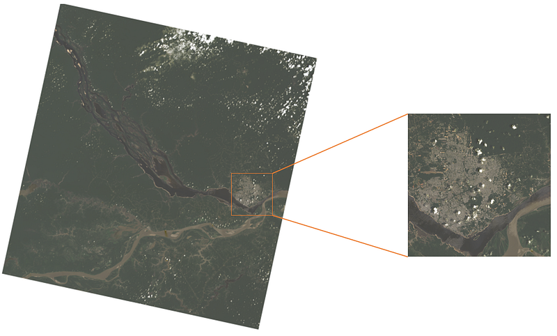
Now that we’ve managed to open a Landsat band, how about trying to open other bands, combine them in a color image or even “zoom” in a specific area, like the examples in Figure 9. But don’t worry if it seems too complicated. Next story we will perform these tasks.

Figure 9: Landsat 8 image from 10/26/2020, presented in natural colors and Manaus city in the zoomed detail. Image by author.

Conclusion

In today’s story we learned the basics of how to install Python and use it to open a band from a Landsat 8 image. In the next story we will learn to work with multiple bands, create indices (such as the NDVI or NDWI) and show images with natural colors and false RGB.

In the meantime, leave in the comments what you thought of the tutorial and if you had any difficulties to follow it, or any suggestions to improve it. This first one was simple, but we will increase the difficulty over the next steps. Stay tuned and see you next time!

Stay Connected

If you liked this article and want to continue reading/learning without limits, consider becoming a Medium member. I’ll receive a portion of your membership fee if you use the following link, with no extra cost to you.

Join Medium with my referral link — Maurício Cordeiro

As a Medium member, a portion of your membership fee goes to writers you read, and you get full access to every story…

cordmaur.medium.com