Illustration of Central Limit Theorem Using Monte-Carlo Simulation

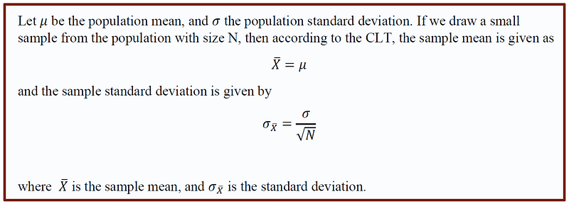
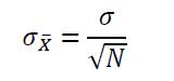
The Central Limit Theorem (CLT) is one of the most important theorems in statistics and data science. The CLT states that the sample mean of a probability distribution sample is a random variable with a mean value given by population mean and standard deviation given by population standard deviation divided by square root of N, where N is the sample size.

We can illustrate the central limit theorem using the uniform distribution. Any probability distribution such as normal, Poisson, Binomial would work as well.

The Uniform Distribution

Lets consider a uniform distribution defined in the range [a, b]. The probability distribution function, mean, and standard deviation are obtained from Wolfram Mathematica Website.

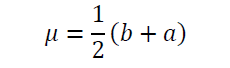
a) Population mean

For a uniform distribution, the population mean is given by

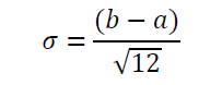
b) Population standard deviation

For a uniform distribution, the population standard deviation is given by

The Central Limit Theorem states that the mean of any sample with size N is a random variable with mean value of

and standard deviation given by

Let us now illustrate our calculation by considering a uniform distribution with a = 0, b = 100. We shall illustrate the Central Limit Theorem by considering the population (N →Infinity) and two samples, one with N = 100, and the other with N = 1000.

I. Analytical Results

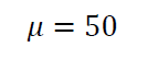
a) Population Mean

Using the equations above, the population mean for a uniform distribution with a = 0, and b = 100 is

b) Population Standard Deviation

Similarly, the population standard deviation of a uniform distribution with a = 0 and b = 100 is

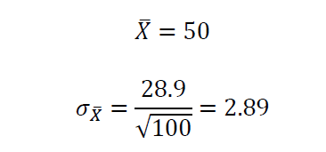
c) Sample 1 with N = 100

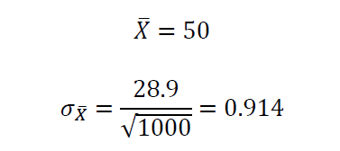
d) Sample 2 with N = 1000

II. Monte-Carlo Simulation Results

For Monte-Carlo simulations, we generate a very large population of size 10,000.

a) Population Mean

pop_mean <- mean(runif(10000,0,100))

Output is 50.0 which agrees with our analytical results.

b) Population Standard Deviation

pop_sd <- sd(runif(10000,0,100))

Output is 28.9 which agrees with out analytical results.

c) Monte-Carlo Code for two Samples with N = 100 and N = 1000

library(tidyverse)

a <-0
b <-100

mean_function <-function(x)mean(runif(x,a,b))

B <-10000

sample_1 <-replicate(B, {mean_function(100)})

sample_2 <-replicate(B, {mean_function(1000)})

Outputs from Monte-Carlo Simulation

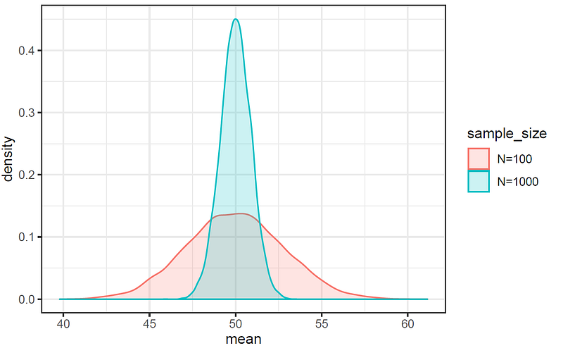
mean(sample_1)

yields 50.0 which is consistent with our analytical results.

sd(sample_1)

yields 2.83 which is consistent with our analytical results (2.89).

mean(sample_2)

yields 50.0 which is consistent with our analytical results.

sd(sample_2)

yields 0.888 which is consistent with our analytical results (0.914).

d) Generate Probability Distributions of the Mean for N = 100 and N = 1000.

X <- data.frame(sample_size=rep(c("N=100","N=1000"),
                times=c(B,B)),mean=c(sample_1,sample_2))

X%>%ggplot(aes(mean,color=sample_size))+
    geom_density(aes(mean,fill=sample_size),alpha=0.2)+
    theme_bw()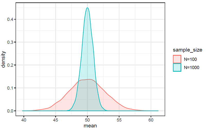

The figure shows that the sample mean is a random variable that is normally distributed with a mean value equal to the population mean, and a standard deviation that is given by the population standard deviation divided by the square root of the sample size. Since the sample standard deviation (uncertainty) is inversely proportional to the sample size, the precision of the calculated mean value decreases with larger sample sizes.

Implications of the Central Limit Theorem

We’ve shown that the sample mean of any probability distribution is a random variable with mean value equal to the population mean and standard deviation of the mean given by:

Based on this equation, we can observe that as the sample size N → Infinity, the uncertainty or standard deviation of the mean goes to zero. This means that the larger the size of our dataset, the better, as larger samples lead to smaller variance error.

In summary, we’ve discussed how the central limit theorem can be proved using Monte-Carlo simulation. The central limit theorem is one of the most important theorems in statistics and data science, so as a practicing data science, familiarity with the mathematical foundations of the central limit theorem is very important.