Profit Like a Pro: A Practical Guide to Backtesting and Optimizing Trading Strategies with Vectorbt

Welcome to the world of trading, where success lies in being able to identify market trends and make profitable trades when the opportunities arise. Technical analysis tools such as Moving Average Convergence Divergence (MACD) can help traders identify potential buy and sell signals. However, to achieve long-term profitability, traders must apply these tools effectively and that requires careful evaluation and optimization.

In this article, we’ll explore how to optimize the MACD trading strategy using python-based Vectorbt package. By conducting a systematic analysis of the strategy over a range of hyperparameters, we’ll uncover the most effective combination of hyperparameters to optimize the strategy for trading in the stock market.

We’ll also evaluate the Sharpe ratio of the MACD strategy using walk forward validation and compare it to a simple buy-and-hold approach. By the end of this article, you’ll have a better understanding of the MACD trading strategy, how to optimize its performance and how to apply it to real-world trading scenarios.

Vectorbt is a high-performance backtesting framework of scalable, composable and extendable pandas-based vectorized backtesting and analysis tools. It allows you to use Pandas DataFrames and Series to model, analyze and execute complex trading strategies.

To get started, let’s import the necessary libraries:

import numpy as np
import pandas as pd
import scipy.stats as stats
import kaleido
import vectorbt as vbt
from itertools import combinations, product

Portfolio configuration

Next, we will set the parameters for our walk forward validation. We will use 30 windows, each 2 years long and with 180 days for testing:

# WalkForward Split params - 30 windows, each 2 years long, 180 days for test
split_kwargs = dict(
    n=20, 
    window_len=365 * 2, 
    set_lens=(180,), 
    left_to_right=False
)

We will also set the Backtesting portfolio parameters, in this example we do not take into account the stop loss, but you can include it to make different tests.

# Stop Loss - Not included in this example
# stop = 0.05  # 5%

# Backtesting Portfolio params
pf_kwargs = dict(
    init_cash=100.,      # 100$ initial cash
    slippage=0.001,      # 0.1%
    fees=0.001,          # 0.1%
    freq='d',
    # direction='both',  # long and short
    # sl_stop=stop,      # Stop Loss
    # sl_trail=True,     # Trailing Stop Loss
)

We will define the hyper-parameter space for our MACD strategy. We will use 49 fast x 49 slow x 19 signal. We could also add two additional parameters (not included in this example), macd_ewm, which will be a Boolean value that determines whether to use exponential moving averages for the MACD indicator:

# Define hyper-parameter space -> 49 fast x 49 slow x 19 signal. To Add: X 2 macd_ewm (np.array([True, False], dtype=bool))
fast_windows, slow_windows, signal_windows = vbt.utils.params.create_param_combs(
    (product, (combinations, np.arange(10, 40, 1), 2), np.arange(10, 21, 1)))

To retrieve the necessary price data, we’ll be using the download() method from YFData to download the historical price data for Bitcoin for this example. In case you prefer specific intervals, feel free to adjust them as needed, but keep in mind that the freq parameter of the portfolio should also be changed accordingly.

# Get BTC Close price from Yahoo Finance
price = vbt.YFData.download('BTC-USD').get('Close') # Valid intervals: [1m, 2m, 5m, 15m, 30m, 60m, 90m, 1h, 1d, 5d, 1wk, 1mo, 3mo]

Now that we have our price data, let’s take a look at the price evolution. We can do this using the plot() method:

# Price evolution
price.vbt.plot().show_png()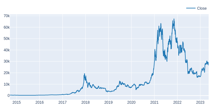

We can also create rolling splits for walk forward validation using the rolling_split() method:

# Rolling splits for Walk Forward Validation
price.vbt.rolling_split(**split_kwargs, plot=True).show_svg()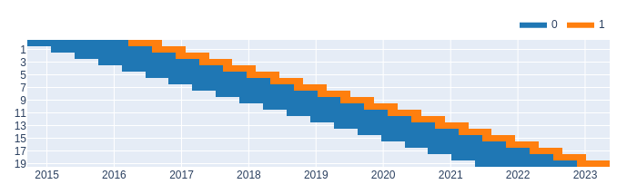

We can see that the price data is split into multiple windows, each of which will be used for validation in our walk forward approach. Now we perform the walk forward validation splits:

# Walk Forward Validation Split
(in_price, in_indexes), (out_price, out_indexes) = price.vbt.rolling_split(**split_kwargs)

print(in_price.shape, len(in_indexes))    # in-sample
print(out_price.shape, len(out_indexes))  # out-sample

(550, 20) 20
(180, 20) 20

Building the Trading Strategy

We will use the MACD indicator to build our trading strategy. The MACD indicator is available in the VectorBT library and can be computed using the vbt.MACD.run() method. The vbt.MACD.run() method takes the fast_window, slow_windowand signal_window arguments to define the number of periods for the fast, slow and signal moving averages, respectively.

We will build a long-only strategy that enters a position when the MACD line is above zero and the signal line and exits the position when the MACD line is below zero or the signal line.

def simulate_all_params_MACD(price, fast_windows, slow_windows, signal_windows, **kwargs):
    # Run MACD indicator
    macd_ind = vbt.MACD.run(price, fast_window=fast_windows, slow_window=slow_windows, signal_window=signal_windows)
    
    # Entry when MACD is above zero AND signal
    entries = macd_ind.macd_above(0) & macd_ind.macd_above(macd_ind.signal) 

    # Exit when MACD is below zero OR signal
    exits = macd_ind.macd_below(0) | macd_ind.macd_below(macd_ind.signal)

    # Build portfolio 
    pf = vbt.Portfolio.from_signals(price, entries, exits,**kwargs)

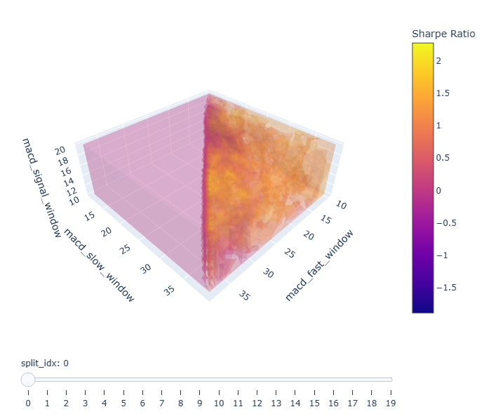
    # Draw all window combinations as a 3D volume
    fig = pf.sharpe_ratio().vbt.volume(
        x_level='macd_fast_window',
        y_level='macd_slow_window',
        z_level='macd_signal_window',
        slider_level='split_idx',
        trace_kwargs=dict(
            colorbar=dict(
                title='Sharpe Ratio', 
            )
        )
    )
    fig.show()

    return pf

We define the simulate_all_params_MACD() function to run the MACD indicator for a range of fast_window, slow_window and signal_window values and simulate the long-only strategy using the resulting signals. The function takes the following arguments:

• price: The price data of the asset.
• fast_windows: A list of fast moving average window sizes to test.
• slow_windows: A list of slow moving average window sizes to test.
• signal_windows: A list of signal moving average window sizes to test.
• **kwargs: Additional arguments to pass to vbt.Portfolio.from_signals(), such as initial_cash, fees and slippage.

We then define the entries and exits signals based on the MACD indicator as described above. We use the vbt.Portfolio.from_signals() method to simulate the long-only strategy and compute the resulting metrics. Finally, we visualize the Sharpe ratio of each combination of hyperparameters using a 3D volume plot.

Once we have defined our simulate_all_params_MACD function, we can call it for any period. Here, we call it for the in_price using the following code.

# Simulate all params for in-sample ranges
in_pf = simulate_all_params_MACD(in_price, fast_windows, slow_windows, signal_windows, **pf_kwargs)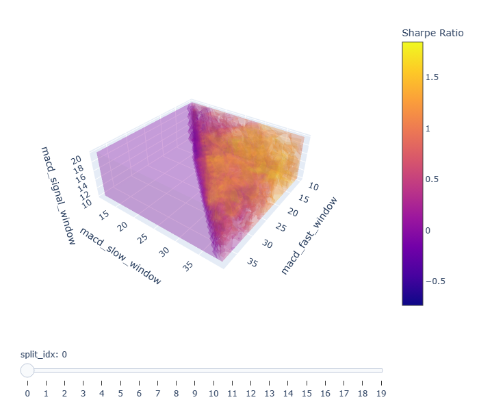

Getting the best hyperparameters for each split

After simulating the portfolio for all hyperparameter combinations and each split, we can obtain the optimal combination’s index that we should use for each split.

# Get Best index - max performance (Sharpe Ratio) by each split
def get_best_index(performance, higher_better=True):
    if higher_better:
        return performance[performance.groupby('split_idx').idxmax()].index
    return performance[performance.groupby('split_idx').idxmin()].index

in_best_index = get_best_index(in_pf.sharpe_ratio())

Here, we have defined get_best_index to return the combination of hyperparameters that yield the highest Sharpe ratio during each period. We determine it by calling the idxmax method on in_pf.sharpe_ratio df grouped by the split number and applied on its index. The result is a multi-index series that contains the index of the Sharpe ratio peak for every split. We then use this series to select the best parameters.

# Get Best params
def get_best_params(best_index, level_name):
    return best_index.get_level_values(level_name).to_numpy()

# Get best params from level values
in_best_fast_windows = get_best_params(in_best_index, 'macd_fast_window')
in_best_slow_windows = get_best_params(in_best_index, 'macd_slow_window')
in_best_signal_windows = get_best_params(in_best_index, 'macd_signal_window')

The above code defines get_best_params as a simple function that returns the values of the level_name column of the best_index series queried by get_level_values and converted to numpy arrays.

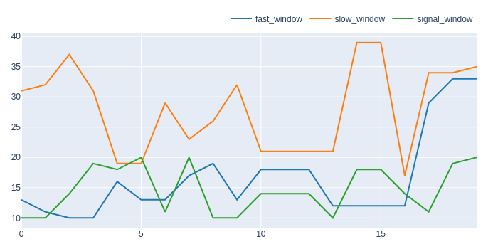
After obtaining the best hyperparameters for each split, we can display the best combination of hyperparameters for the in-sample data.

# Show best
in_best_window_combs = np.array(list(zip(in_best_fast_windows, in_best_slow_windows, in_best_signal_windows)))
pd.DataFrame(in_best_window_combs, columns=['fast_window', 'slow_window', 'signal_window']).vbt.plot().show_svg()

The code above creates an array of the best hyperparameter combinations and then plots them using the vbt.plot() function.

We can use the in_best_index series, which contains the indices of the optimal combinations, to select the best combination of hyperparameters by split.

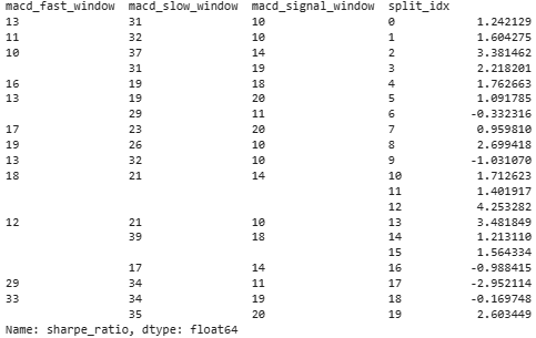
# First five best combinations
in_best_index[:5]

Here, we have printed the first five rows:

MultiIndex([(13, 31, 10, 0),
            (11, 32, 10, 1),
            (10, 37, 14, 2),
            (10, 31, 19, 3),
            (16, 19, 18, 4)],
           names=['macd_fast_window', 'macd_slow_window', 'macd_signal_window', 'split_idx'])

In-sample data performance Analysis

To further analyze the performance of the selected hyperparameters, we can obtain the statistics of the portfolio for a specific combination of hyperparameters. We will show the statistics of the combination with the highest Sharpe ratio during the first split.

# Get stats of the first best combination
print(in_pf[(13, 31, 10, 0)].stats())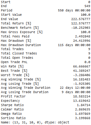

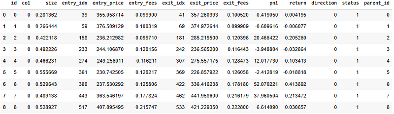
We can also obtain the trades records of the portfolio using the same combination of hyperparameters using the following code:

# Get Trades
display(in_pf[(13, 31, 10, 0)].trades.records)

The code above displays the trades made by the portfolio using the first best combination of hyperparameters.

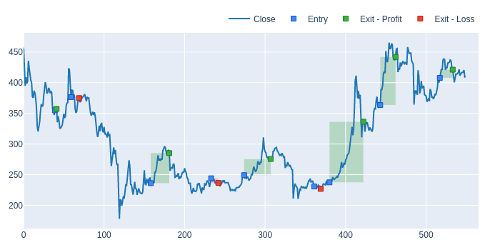
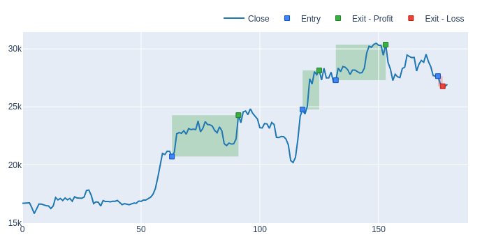
Lastly, we can plot the trades made by the portfolio on the price chart:

# Plot Trades
in_pf[(13, 31, 10, 0)].trades.plot().show_svg()

The code above produces a plot that shows the trades entry and exit points.

Sharpe Ratio with a Buy&Hold strategy for each data split

Before we can evaluate the out-of-sample Sharpe ratio of our MACD strategy, we need a benchmark to compare against. To do this, we can simulate a buy-and-hold trading strategy on each data split and calculate the Sharpe ratio for each benchmark.

# Simulate buy-and-hold function
def simulate_holding(price, **kwargs):
    pf = vbt.Portfolio.from_holding(price, **kwargs)
    return pf.sharpe_ratio()

# In-sample Sharpe Ratio with buy-and-hold
in_hold_sharpe = simulate_holding(in_price, **pf_kwargs)

# Out-sample Sharpe Ratio with buy-and-hold
out_hold_sharpe = simulate_holding(out_price, **pf_kwargs)

This code first defines a function simulate_holding that creates a portfolio signal that holds the asset over the entire period and then computes the Sharpe ratio using the resulting portfolio. We call this function for both in_price and out_price.

Simulate all MACD params for out-sample ranges

We use the same function simulate_all_params_MACD to simulate MACD performance in the out-sample range using all possible combinations of hyperparameters.

# Simulate all MACD params for out-sample ranges
out_pf = simulate_all_params_MACD(out_price, fast_windows, slow_windows, signal_windows, **pf_kwargs)

This function outputs the portfolio performance for all the possible hyperparameter combinations and computes the Sharpe ratio using the portfolio.

Simulate best params MACD for out-sample ranges

After finding the optimal hyperparameters for the in-sample data, we use them to simulate the MACD performance for the out-sample range. However, since there is only one parameter combination per split, we do not include the 3D volume plot as it would not provide any additional information.

def simulate_best_params_MACD(price, in_best_fast_windows, in_best_slow_windows, in_best_signal_windows, **kwargs):
    # Run MACD indicator - per_column=True for one combination per column.
    macd_ind = vbt.MACD.run(price, fast_window=in_best_fast_windows, slow_window=in_best_slow_windows, signal_window=in_best_signal_windows, per_column=True)
    
    # Long when MACD is above zero AND signal
    entries = macd_ind.macd_above(0) & macd_ind.macd_above(macd_ind.signal) 
    
    # Short when MACD is below zero OR signal
    exits = macd_ind.macd_below(0) | macd_ind.macd_below(macd_ind.signal)
    
    # Build portfolio 
    pf = vbt.Portfolio.from_signals(price, entries, exits, **kwargs)
       
    return pf

# Use best params from in-sample ranges and simulate them for out-sample ranges
out_test_pf = simulate_best_params_MACD(out_price, in_best_fast_windows, in_best_slow_windows, in_best_signal_windows, **pf_kwargs)
print(out_test_pf.sharpe_ratio())

Here, simulate_best_params_MACD uses the optimal combination of hyperparameters found during the in-sample validation and applies them to the out-sample range. It produces an out-of-sample test that returns the Sharpe ratio for each split:

Out-sample data performance analysis

We can call out_test_pf.stats() to print the statistics of the last combination of hyperparameters (most recent data), which is the optimal combination found using the in-sample data.

# Get stats of the last best combination
print(out_test_pf[(33, 35, 20, 19)].stats())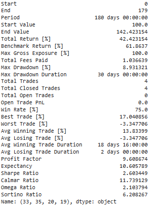

Next, we displayed the trades of this best combination of hyperparameters, as simulated on the out-sample data.

# Get Trades
display(out_test_pf[(33, 35, 20, 19)].trades.records)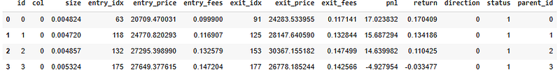

In order to gain a better understanding of the trades, we also visualized the entry and exit points on the price chart of the latest split, allowing us to visualize the actual buy and sell signals generated by the MACD strategy in action.

# Get Trades
out_test_pf[(33, 35, 20, 19)].trades.plot().show_svg()

This code produces a plot that shows the trades’ entry and exit points for the optimal combination of hyperparameters during the last split of the out-sample data.

Comparing the buy-and-hold and MACD strategies

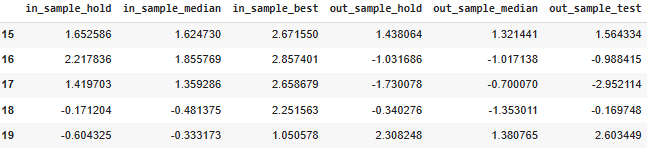
Finally, we compared the performance of the MACD strategy to a simple buy-and-hold approach using the cv_results_df dataframe.

# In-sample and Out-sample results DF
cv_results_df = pd.DataFrame({
    'in_sample_hold': in_hold_sharpe.values,
    'in_sample_median': in_pf.sharpe_ratio().groupby('split_idx').median().values,
    'in_sample_best': in_pf.sharpe_ratio()[in_best_index].values,
    'out_sample_hold': out_hold_sharpe.values,
    'out_sample_median': out_pf.sharpe_ratio().groupby('split_idx').median().values,
    'out_sample_test': out_test_pf.sharpe_ratio().values
})

The DataFrame compares the Sharpe ratios obtained with a buy-and-hold strategy to the Sharpe ratios obtained with a MACD strategy. We calculated the Sharpe ratio for each split of the in-sample and out-sample data and then computed three types of Sharpe ratios:

• Sharpe Ratio using Buy-and-Hold: This is the Sharpe ratio of the simple buy-and-hold strategy for every split.
• Median Sharpe Ratio: This is the median Sharpe ratio over all the combinations of hyperparameters.
• Best Sharpe Ratio: This is the Sharpe ratio for the best combination of hyperparameters.

Below are the five last rows of this DataFrame:

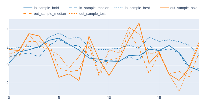
Afterwards, we plot the results dataframe, representing buy-and-hold Sharpe ratios to the median and best Sharpe ratios for the MACD strategy for both in-sample and out-sample data.

color_schema = vbt.settings['plotting']['color_schema']

cv_results_df.vbt.plot(
    trace_kwargs=[
        dict(line_color=color_schema['blue']),
        dict(line_color=color_schema['blue'], line_dash='dash'),
        dict(line_color=color_schema['blue'], line_dash='dot'),
        dict(line_color=color_schema['orange']),
        dict(line_color=color_schema['orange'], line_dash='dash'),
        dict(line_color=color_schema['orange'], line_dash='dot')
    ]
).show_svg()

The plot has six lines:

• Blue solid line: median Sharpe Ratio or MACD for in-sample data.
• Blue dotted line: best combination of hyperparameters or MACD for in-sample data.
• Blue dashed line: Sharpe Ratio using Buy-and-Hold for in-sample data.
• Orange solid line: median Sharpe Ratio or MACD for out-sample data.
• Orange dotted line: best combination of hyperparameters or MACD for out-sample data.
• Orange dashed line: Sharpe Ratio using Buy-and-Hold for out-sample data.

This visualization allows us to evaluate the performance of the buy-and-hold strategy against the MACD trading strategy and assess the robustness of the MACD strategy through its median and best Sharpe ratios over all the combinations of hyperparameters.

Conclusion

The MACD trading strategy is one of the most popular technical analysis tools and this analysis confirms that it can be effective in trading with the right hyperparameters. By analyzing the performance of the MACD strategy against the simple buy-and-hold approach, we have shown that it does deliver better results on average, although its performance on out-of-sample data was lower compared to the in-sample data.

This comprehensive analysis also confirms the effectiveness of the python-based Vectorbt package in backtesting trading strategies and evaluating their performance. Vectorbt is an efficient and straightforward tool that enables traders and data analysts to perform in-depth strategy analyses easily.

Overall, the MACD trading strategy has its unique benefits and limitations and traders must be careful when applying it to real-world trading. Nevertheless, this study provides a robust framework for assessing hyperparameters, optimizing and evaluating the performance of the MACD strategy, providing a powerful tool to traders seeking long-term profitability.

Subscribe to DDIntel Here.

Visit our website here: https://www.datadriveninvestor.com

Join our network here: https://datadriveninvestor.com/collaborate