Probabilistic machine learning in 5 minutes, an intuition.

Summary

Probabilistic machine learning is presented as a critical advancement to improve the predictive capabilities of models by considering multiple hypotheses and avoiding overfitting, with Bayesian methods as a central approach.

Abstract

The article introduces the concept of probabilistic machine learning, emphasizing its importance as neural networks become more prevalent in production. It argues that traditional neural network models, which are based on a single set of weights (W), may lead to overfitting due to their inability to capture the full distribution of possible explanations for the data. The author suggests that by adopting a Bayesian approach and considering a range of hypotheses, each weighted by its posterior probability, one can better predict new data by using the posterior predictive distribution. This approach acknowledges that a dataset is a sample from a complex joint probability distribution and that multiple sets of weights could explain the data. The article also touches on the challenges of high-dimensional, non-convex optimization in neural networks and hints at future discussions on Bayesian model selection and techniques like Markov Chain Monte Carlo for sampling from the posterior distribution.

Opinions

The author believes that the current trend of using neural networks in production may lead to overfitting due to their reliance on a single hypothesis (set of weights).
There is a suggestion that the field should move beyond the "plug-in approximation" of delivering a single set of parameter values as the solution.
The article conveys that life is not simple and that the problem of optimizing neural network weights is complex, often leading to local optima rather than the best hypothesis.
The author has a positive view of Bayesian methods, implying that they provide a more robust framework for machine learning by incorporating prior knowledge and considering multiple hypotheses.
There is an acknowledgment that while Bayesian methods are powerful, they are also computationally expensive and complex, which is why they have not been widely implemented in production.
The author encourages readers to consider the theoretical joint probability distribution from which datasets are derived, suggesting that understanding this distribution is key to learning the true tendencies of the data.
The article expresses excitement about the potential of probabilistic machine learning and encourages readers to have fun and continue learning about these advanced techniques.

Maybe you have not heard about probabilistic machine learning, but as soon as Bayesian models will be implemented into production, it will be a critical, yet difficult, concept to know.

The reverend Thomas Bayes, mostly known by its Bayes (or Laplace) Theorem makes us rethink machine learning.

Introduction

Everyone is so happy with neural networks in production, they provide predictive power, and are trendy. However, their productions may not be the best explanation, or better, the unique explanation, for a plethora of different data problems. Remember, neural networks are essentially models that are parametrized by a tensor W of weights. I do not pretend to be here very technical and you may wonder why I am speaking about this, but please just keep reading and do not be afraid. The optimizer of the neural network, via the backpropagation algorithm, estimate some tensor values such that they minimize a loss function L(W) over a particular dataset D. Oh, life is very happy and this is easy… well.. you may be suffering from overfitting…

Overfitting emerges when we do not learn the tendency, but the spurious details of our particular sample that do not explain the tendency of the data. (Photo: https://www.analyticsvidhya.com/blog/2020/02/underfitting-overfitting-best-fitting-machine-learning/)

The problem with a plug-in approximation

If you think about it, your W solution is just one hypothesis that explains your dataset D according to the assumptions of your model M, your neural network. In probabilistic machine learning, we call that a “plug-in approximation”, just delivering one set of parameter values as the final solution instead of considering more hypothesis (set of parameter values) that explains the data. In other works, the likelihood of W given M and the data D is high. But life is not that simple. The problem of optimizing the weights of a neural network is high-dimensional, non-convex and multi-modal. The gradient of the loss function with respect to the parameters is very expensive and approximations such as the one done by stochastic gradient descent are very common. Consequently, it is practically impossible that the final solution found by these algorithms represent the best hypothesis that explains our data under the assumptions of the neural network. It may only be a local optima, or a point near the local optima. Hence, more hypotheses would be likely, and not using them to predict new data conditioned to previous data can lead to overfitting. Your k-fold cross validation may help to avoid this, but you can never know whether all your dataset is representative of the target population, or theoretical probability distribution where your dataset comes from. Wow, I am sounding Bayesian here, and that is precisely what I pretend ;-).

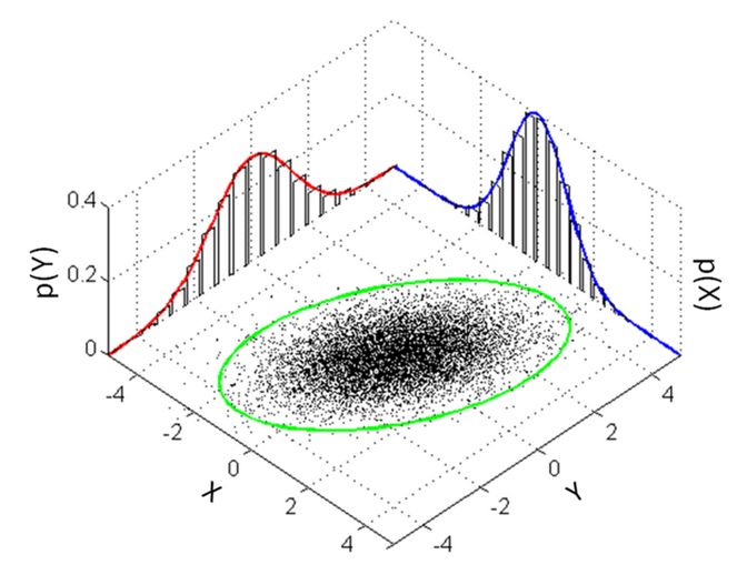
A dataset is a sample of a joint theoretical probability distribution p(y,X)

Because the truth is that your dataset D is just a sample from a complex theoretical joint probability distribution p(y,X) between the target variable y and the explanatory variables X. And the assumptions of the model, such as a neural network, that we are using to get a parametric solution of that joint probability distribution p(y,X )must satisfy the properties of the data. If it satisfies such properties, several hypothesis W, the parameters of the neural network, may have similar likelihood about the data p(y,X|W). The only way to take them all into account is to compute a posterior probability distribution of the parameters with respect to the data p(W|y,X), with the famous Bayes theorem! Where the prior distribution encodes the assumptions that we make about the parameters of the model, in this case, the weights of the neural network.

For any dataset, we can think on a theoretical joint probability distribution that, for any X, has a conditional probability distribution of the target y. It is the distribution that has generated that data. The tendency that we want to learn.

And how do I predict, then?

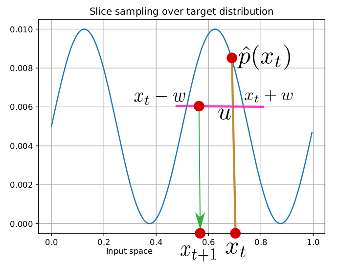
Basically, you can use the posterior probability distribution of the parameters of the neural network p(W|y,X) to make a prediction of all the neural networks parametrized with different W and weighted according to p(W|y,X). Instead of just using one neural network parametrized by W, estimated via k-fold CV, we use samples from p(W|y,X), weighted by p(W|y,X) to approximate the true prediction of the whole model, the posterior predictive distribution: p(y) = ∫ p(y|W,X) p(W|y,X) dW. Just observe that in machine learning we just substitute p(W|y,X) by W found by k-fold CV. That is called the plug-in approximation, that is very prone to overfitting. We can approximate p(y) by sampling from p(W|y,X) and do the mean of the predictions using some sampling Markov Chain Monte Carlo technique. I will write another post about it ;-).

Sampling from a probability distribution about the parameters or any other quantity can be done using a plethora of techniques. Here, the slice sampling slices the distribution to find areas with high probability to obtain samples from a distribution.

How do I know how good is my model?

But how do I do model selection under this framework? Easy, in essence, you must do an expectation (which is a generalization of the empirical mean to the population) about the likelihood of every possible hypothesis and your prior beliefs. The mean of all the likelihoods of the model. That is the marginal likelihood of the data p(X,Y) = ∫ p(X,Y|W)p(W) dW. This is a number, the bigger the best.

It is Bayesian model selection. Unfortunately, it is very costly to obtain these quantites. But to overcome this issue, we will leave that for a future article. Remember to have fun in your work if it is possible and never stop reading!