Summary

The web content discusses the use of probabilistic forecasts, particularly quantile forecasts, and the pinball loss function to optimize supply chain and inventory management, emphasizing the importance of evaluating forecast accuracy with asymmetrical penalties.

Abstract

The article on the website delves into the concept of probabilistic forecasting, highlighting its significance in improving supply chain efficiency and setting inventory targets. It introduces the pinball loss function as a tool for assessing the accuracy of quantile forecasts, which are probabilistic in nature and aim to predict a specific demand quantile. The pinball loss function is designed to penalize under forecasting more severely than over forecasting, reflecting the asymmetrical impact of forecasting errors in different contexts, such as high-margin products where understocking can be more detrimental than overstocking. The article also distinguishes between forecasting the median and the mean demand, noting that optimizing for the Mean Absolute Error (MAE) leads to forecasting the median demand. Additionally, the article provides a self-assessment quiz to reinforce understanding and concludes with a Python implementation of the pinball loss function, offering practical insights for readers interested in applying these concepts.

Opinions

The author suggests that over forecasting is less problematic than under forecasting when dealing with high-margin products, advocating for aiming at a high demand quantile when setting safety stock targets.
There is an emphasis on the importance of understanding the difference between forecasting the median and the mean, with a clear preference for the median when optimizing MAE.
The article promotes the use of the pinball loss function for evaluating quantile forecasts, arguing that it provides a more nuanced assessment of forecast accuracy by considering the asymmetrical nature of forecasting errors.
The author provides a Python code snippet for the pinball loss function, indicating a commitment to practical, actionable advice for readers looking to implement these concepts in their work.
The article implies that traditional safety stock formulas can be seen as a special case of quantile forecasting, integrating the concept of the Gaussian alpha quantile.
By including a self-assessment quiz and providing answers with explanations, the author conveys a dedication to reader engagement and education on the topic of probabilistic forecasting.

Probabilistic Forecasts: Pinball Loss Function

Probabilistic forecasts are essential to optimize supply chains and inventory targets. How can we evaluate the quality of probabilistic forecasts?

Self-Assessment Quiz

Let’s start with a few questions. Read them first before going through the article. By the end of your reading, you should be able to answer them. (The answers are provided at the end as well as a Python implementation)

You want to forecast your product’s demand. Specifically, you want to predict a value for which the demand has an 80% probability of being under. What is the worst, over forecasting the actual demand or under forecasting it?
You design a forecast model that reduces the absolute error (or MAE). Is your model aiming for the average demand or the median demand?
You made a 95% quantile demand forecast, your forecast was 150, and the observed demand is 120. How would you assess the quality of your forecast?
You sell high-margin products. What is the worst: overstocking or understocking them? When setting the safety stock target, should you aim for a high or a low demand quantile?

Probabilistic Forecasting and Inventory Optimization

Forecasts should only be made to help you making the right supply chain decisions.

towardsdatascience.com

Quantile Forecasts

A quantile forecast is a probabilistic forecast aiming at a specific demand quantile (or percentile).

Definition: Quantile

The quantile α (α is a percentage, 0<α<1) of a random distribution is the value for which the probability for an occurrence of this distribution to be below this value is α.

P(x<=Quantile) = α

In other words, the quantile is the distribution’s cumulative distribution function evaluated at α.

Quantile α = F^{-1}(α)

In simple words, if you do an 80% quantile forecast of tomorrow’s weather, you would say, “There is an 80% probability that the temperature will be 20°C or lower.”

Side note: If you are used to inventory optimization and the usual safety stock formula

Ss = z * σ * √(R+L)

z is the gaussian alpha quantile z=Φ^(-1) (α). Somehow, you can see the safety stock formula as the α quantile forecast of the demand over the risk-horizon. PS: Remember to include the review period in this formula.

Asymmetrical Penalties

How can we assess the accuracy of a quantile forecast? Let’s take another look at our above example: you forecast that tomorrow’s 80th temperature quantile is 20°C. The next day, the temperature is 16°C.

How accurate was your forecast?

Before discussing the math, let’s get an intuition on how we should evaluate (or penalize) a quantile forecast. Somehow, when we say, “We forecast the temperature to have 80% of chances to be below 20°C,” we expect the temperature to be lower than 20°C and would be surprised that the temperature would be 25°C.

In other words, this quantile forecast should get a higher penalty if it under forecasted the temperature than if it overpredicted it.

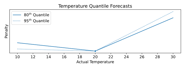
Moreover, as shown in the figure above, the penalty for over forecasting should be even higher for higher quantiles. For example, if your 95% temperature quantile forecast is 20°C, you would be very surprised if the actual temperature was 25°C.

Pinball Loss Function

Let’s formalize this forecasting penalty using the pinball loss function (or quantile loss function).

The pinball loss function L_α is computed for a quantile α, the quantile forecast f, and the demand d as

L_α (d,f) = (d-f) α    if d≥f
            (f-d)(1-α) if f>d

This loss function aims to provide a forecast with an α probability of under forecasting the demand and an (α-1) probability of over forecasting the demand.

Intuition and Examples

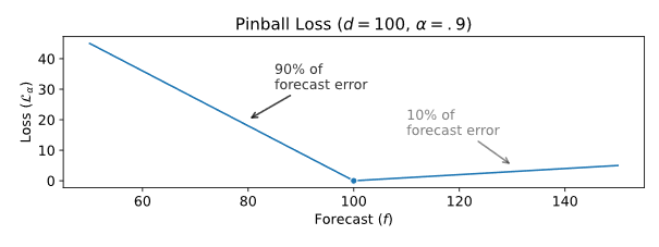
Let’s see how the pinball function works in practice. In the figure below, you can see an example with d=100 and α=90% (we want to forecast the demand 90th quantile) where the pinball loss function L_α is computed for different values of f.

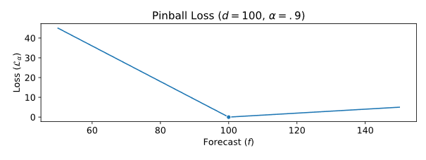
As you can see, the pinball loss L_α is highly asymmetrical: it doesn’t increase at the same speed if you over forecast (low penalty) or under forecast (high penalty).

Let’s take an example: forecasting 20 units too much will result in a loss of 10%|f-d|=2 (that is to say that over forecasting is not much penalized). But, on the other side, forecasting 20 units too little will result in a loss of 90%|f-d|=18.

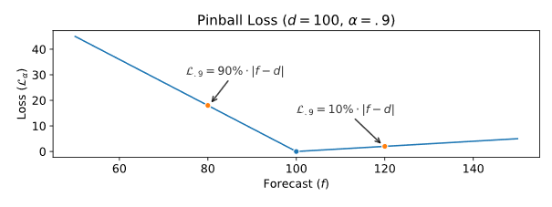
Basically, under forecasting is penalized by α|e| (where e is the forecast error), whereas over forecasting is penalized by (1-α)|e|.

Mean Absolute Error

In my forecasting KPIs article, I highlighted that optimizing the forecast mean absolute error (MAE) will ultimately aim at forecasting the median demand.

Forecast KPI: How to Assess the Accuracy of a Product Portfolio?

How to assess the forecast accuracy when you deal with thousands of SKUs?

towardsdatascience.com

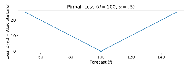
As you can see in the figure below, the 50% quantile pinball loss function corresponds to the regular absolute error — they are interchangeable. Keep in mind that, by definition, forecasting the 50% demand quantile is the same as predicting the demand median. This is another illustration that optimizing the MAE will result in a forecast aiming at the demand median (and not the demand average).

Self-Assessment Solutions

You want to forecast your product’s demand. Specifically, you want to predict a value for which the demand has an 80% probability of being under. What is the worst, over forecasting the actual demand or under forecasting it?

Underforecasting the demand is the worst. If you want to forecast the 80th quantile, you should aim for a value that is likely to be higher than the observed value.

2. You design a forecast model that reduces the absolute error (or MAE). Is your model aiming for the average demand or the median demand?

Optimizing the Mean Absolute Error will ultimately result in forecasting the expected median demand and not the expected mean demand.

3. You made a 95% quantile demand forecast, your forecast was 150, and the observed demand is 120. How would you assess the quality of your forecast?

You can compute the pinball loss of your quantile forecast. Your forecast has an absolute error of 30 units (=|150–120|), and it is an overprediction, so you pinball loss is 1.5 units (=30*0.05%).

4. You sell high-margin products. What is the worst: overstocking or understocking them? When setting the safety stock target, should you aim for a high or a low demand quantile?

You want to have a lot of stock of high-margin products, so understocking them is a bad decision. Henceforth, when setting the stock target you should aim for a high demand quantile.

🐍 Do It Yourself

You can easily implement the pinball loss function in Python in a single expression (with a few modifications compared to the original equation).

def pinball_loss(d, f, alpha):

return max(alpha*(d-f), (1-alpha)*(f-d))