Principal Component Analysis (PCA) with Scikit-learn

Unsupervised Machine Learning Algorithm for Dimensionality Reduction

Hi everyone! This is the second unsupervised machine learning algorithm that I’m discussing here. This time, the topic is Principal Component Analysis (PCA). At the very beginning of the tutorial, I’ll explain the dimensionality of a dataset, what dimensionality reduction means, the main approaches to dimensionality reduction, the reasons for dimensionality reduction and what PCA means. Then, I will go deeper into the topic of PCA by implementing the PCA algorithm with the Scikit-learn machine learning library. This will help you to easily apply PCA to a real-world dataset and get results very fast.

In a separate article (not in this one), I will discuss the mathematics behind the principal component analysis by manually executing the algorithm using the powerful numpy and pandas libraries. This will help you to understand how PCA really works behind the scenes.

What is dimensionality reduction?

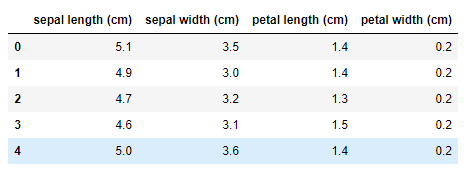
Before we consider reducing the dimensionality of a dataset, we should learn what the dimensionality of a dataset is. Simply, dimensionality is the number of input features (variables) in a dataset. Often, it can be thought as the number of columns (except the label column) in a dataset. The following table shows a part of the iris dataset which contains four features. So, the number of dimensions is four. This means, for example, to demonstrate the first data point in the four-dimensional space, we use p1(5.1, 3.5, 1.4, 0.2) notation.

Dimensionality reduction means reducing the number of features in a dataset.

Main approaches to dimensionality reduction

There are two main approaches to dimensionality reduction:

• Linear methods
• Non-linear methods (Manifold learning)

In this tutorial, I’ll focus on principal component analysis which falls under the category of linear methods.

The curse of dimensionality

The curse of dimensionality arises when we’re working with very high-dimensional datasets. A large number of features requires a lot of computer resources, and a longer period of time to train. The calculations between the data points will become complex and harder when the number of dimensions is very high in the data. That kind of problem is often referred to as the curse of dimensionality in the context of machine learning.

Dimensionality reduction techniques can effectively address the curse of dimensionality. Once the dimensionality has been reduced, machine learning algorithms will be able to perform calculations very effectively and efficiently during training.

What is principal component analysis (PCA)?

PCA is a linear dimensionality reduction technique. It transforms a set of correlated variables (p) into a smaller k (k<p) number of uncorrelated variables called principal components while retaining as much of the variation in the original dataset as possible.

PCA takes advantage of existing correlations between the input variables in the dataset and combines those correlated variables into a new set of uncorrelated variables.

PCA is an unsupervised machine learning algorithm as it does not require labels in the data.

Feature scaling in PCA

PCA requires feature scaling if there is a significant difference in the scale between the features of the dataset; for example, one feature ranges in values between 0 and 1 and another between 100 and 1,000. This is because PCA components are highly sensitive to the relative ranges of the original features [Ref: Hands-On Unsupervised Learning Using Python by Ankur A. Patel] and PCA will attempt to capture the variance that occurred due to relative ranges, not the true variance between the features. We can apply z-score standardization to get all features into the same scale by using Scikit-learn StandardScaler() class which is in the preprocessing submodule in Scikit-learn.

PCA with Scikit-learn

Now, let’s work on an example to see how to implement PCA using Scikit-learn library. For this example, we will use Scikit-learn built-in breast_cancer dataset which contains 30 features and 569 observations. The following steps describe the process of implementing PCA to the dataset with Scikit-learn.

Step 1: Import libraries and set plot styles

As the first step, we import various Python libraries which are useful for our data analysis, data visualization, calculation and model-building tasks. When importing those libraries, we use the following conventions.

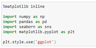
Note that we haven’t imported any Scikit-learn class or function yet. We import them one by one when we need to use them.

Step 2: Get and prepare data

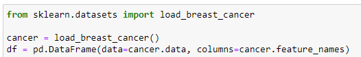
The dataset that we use here is available in Scikit-learn. But it is not in the correct format that we want. So, we have to do some manipulations to get the dataset ready for our task. First, we load the dataset using Scikit-learn load_breast_cancer() function. Then, we convert the data into a pandas DataFrame which is the format we are familiar with.

Now, the variable df contains a pandas DataFrame of the breast_cancer dataset. We can see its first 5 rows by calling the head() method. The following image shows a part of the dataset.

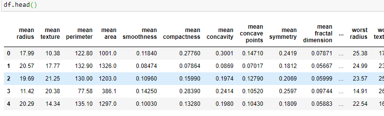
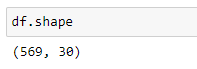
The full dataset contains 30 columns and 569 observations.

Step 3: Apply PCA

In our breast_cancer dataset, the original feature space has 30 dimensions denoted by p. PCA will transform (reduce) data into a k number of dimensions (where k << p) while keeping as much of the variation in the original dataset as possible. These k dimensions are known as the principal components.

By applying PCA, we will be able to visualize high-dimensional data on a 2d or 3d plot, if we choose the number of principal components as 2 or 3. This is the major application of PCA in machine learning.

3.a: Obtain the feature matrix

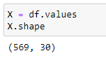
The feature matrix contains the values of all 30 features in the dataset. It is a 569x30 two-dimensional Numpy array. It is stored in the X variable.

3.b: Standardize the features if necessary

You can see that the values of the dataset are not equally scaled. So, we need to apply z-score standardization to get all features into the same scale. For this, we use Scikit-learn StandardScaler() class which is in the preprocessing submodule in Scikit-learn.

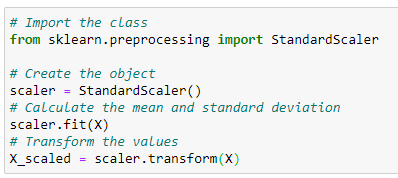
First, we import the StandardScaler() class. Then, we create an object of that class and store it in the variable scaler. Then we use the scaler object’s fit() method with the input X (feature matrix). This will calculate the mean and standard deviation for each variable in the dataset. Finally, we do the transformation with the transform() method of the scaler object. The transformed (scaled) values of X are stored in the variable X_scaled which is also a 569x30 two-dimensional Numpy array.

3.c: Choose the right number of dimensions (k)

Now, we are ready to apply PCA to our dataset. Before that, we need to choose the right number of dimensions (i.e., the right number of principal components — k). For this, we apply PCA with the original number of dimensions (i.e., 30) and see how well PCA captures the variance of the data.

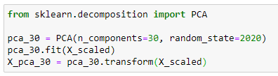
In Scikit-learn, PCA is applied using the PCA() class. It is in the decomposition submodule in Scikit-learn. The most important hyperparameter in that class is n_components. It can take one of the following types of values.

• None: This is the default value. If we do not specify the value, all components are kept. In our example, this exactly the same as n_components=30.
• int: If this is a positive integer like 1, 2, 30, 100, etc, the algorithm will return that number of principal components. The integer value should be less than or equal to the original number of features in the dataset.
• float: If 0 < n_components < 1, PCA will select the number of components such that the amount of variance that needs to be explained. For example, if n_components=0.95, the algorithm will select the number of components while preserving 95% of the variance in the data.

When applying PCA, all you need to do is to create an instance of the PCA() class and fit it using the scaled values of X. Then apply the transformation. The variable X_pca_30 stores the transformed values of the principal components returned by the PCA() class. X_pca_30 is a 569x30 two-dimensional Numpy array.

We have set n_components=30. The original number of dimensions in our dataset is also 30. We have not reduced the dimensionality, and therefore, the percentage of variance explained by 30 principal components should be 100%.

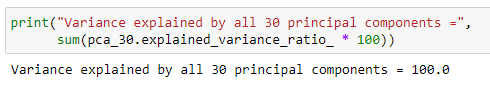
The explained_variance_ratio_ attribute of the PCA() class returns a one-dimensional numpy array which contains the values of the percentage of variance explained by each of the selected components.

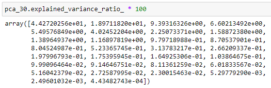
The first component alone captures about 44.27% of the variability in the dataset and the second component alone captures about 18.97% of the variability in the dataset and so on. Also, note that the values of the above array are sorted in descending order. Taking the sum of the above array will return the total variance explained by each of the selected components.

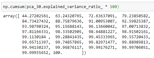
If we get the cumulative sum of the above array, we can see the following array.

Then we create the following plot.

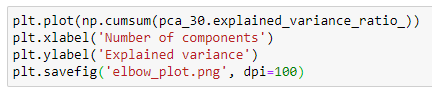
The output is:

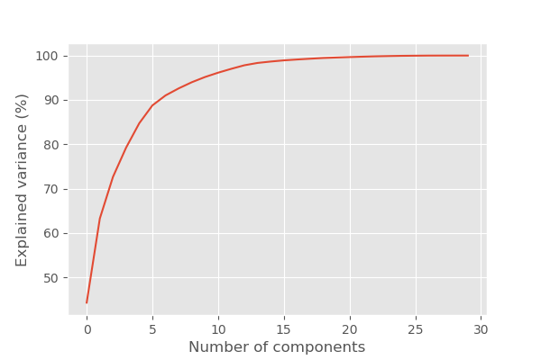
You can see that the first 10 principal components keep about 95.1% of the variability in the dataset while reducing 20 (30–10) features in the dataset. That’s great. The remaining 20 features only contain less than 5% of the variability in data.

It is not possible to create a scatterplot for our breast_cancer dataset because it contains 30 features. Reducing the number of dimensions to two or three makes it possible to create a 2d scatterplot or 3d scatterplot which helps us to detect patterns such as clusters in our dataset. Therefore, dimensionality reduction is extremely useful for data visualization. But, keep in mind that, in our problem, if we create a 2d scatterplot using the first 2 principal components, it only explains about 63.24% of the variability in data and if we create a 3d scatterplot using the first 3 principal components, it only explains about 72.64% of the variability in data!

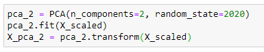
3.d: Apply PCA by setting n_components=2

Let’s apply PCA again to our dataset with n_components=2. This will transform our original data onto a two-dimensional space. This will return 2 components that capture 63.24% of the variability in data as I said earlier.

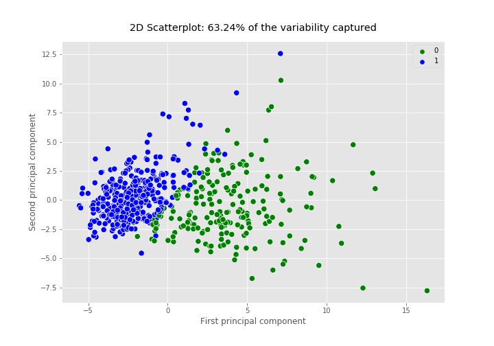
Now, we create a 2d scatterplot of the data using the values of the two principal components.

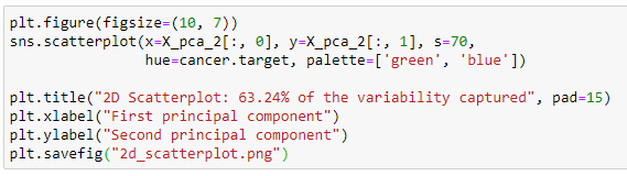
The output is:

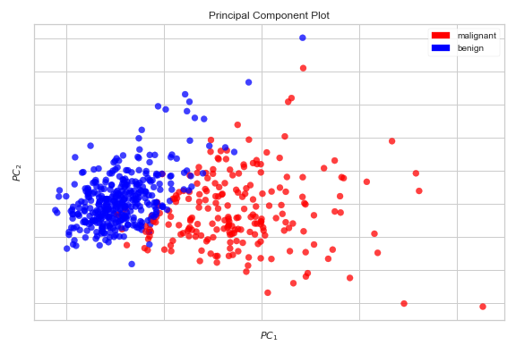
Another way to create the above 2d scatterplot is to use the Yellowbrick machine learning visualization library. Using the PCA Visualizer (an object that learns from data to produce a visualization), we can create an even more informative 2d scatterplot with a just few lines of code.

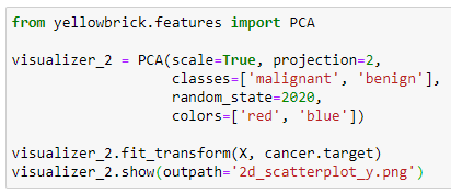
The output is:

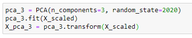
3.e: Apply PCA by setting n_components=3

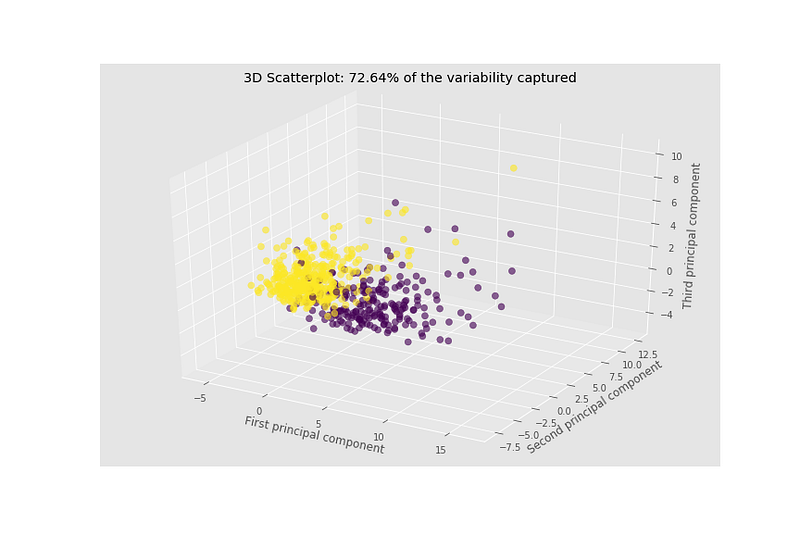
Let’s apply PCA to our dataset with n_components=3. This will transform our original data onto a three-dimensional space. This will return 3 components that capture 72.64% of the variability in data as I said earlier.

Now, we create a 3d scatterplot of the data using the values of the three principal components.

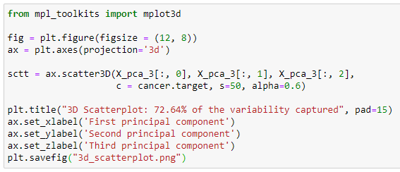
The output is:

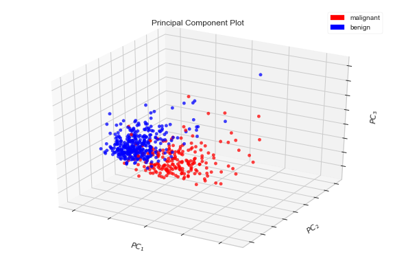
Again we can use the Yellowbrick machine learning visualization library to create the same scatter plot. Using the PCA Visualizer (an object that learns from data to produce a visualization), we can create an even more informative 3d scatterplot with a just few lines of code.

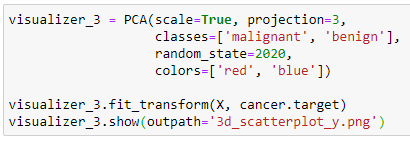
The output is:

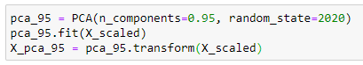
3.f: Apply PCA by setting n_components=0.95

Let’s apply PCA to our dataset with n_components=0.95. This will select the number of components while preserving 95% of the variability in the data.

The shape of the X_pca_95 array is:

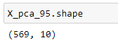
This means that the algorithm has found 10 principal components to preserve 95% of the variability in the data. The X_pca_95 array holds the values of all 10 principal components.

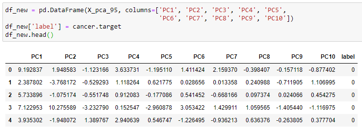
Let’s create a pandas DataFrame using the values of all 10 principal components and add the label column of the original dataset.

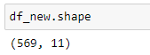
The size of the df_new including the label column is:

When we compare with the original dataset that has 30 features, this contains only 10 features, but with 95% of the variability in data. For future reference, we can save our new dataset as an Excel or CSV file. By setting index=False, the row index labels are not saved in the files.

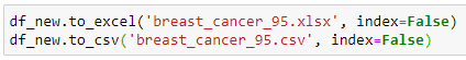
After executing the above code, the files will be saved in your current working directory. By using the new (transformed) dataset, you can apply classification algorithms like Logistic Regression, Support Vector Machines and K-Nearest Neighbours to further analyze the data.

That’s it. In the next article, I will discuss the mathematics behind the principal component analysis by manually executing the algorithm using the powerful numpy and pandas libraries. This will help you to understand how PCA really works behind the scenes.

This is the end of today’s post.

See you in the next story. Happy learning to everyone!

Special credits go to the authors of the following two books which I referred to get the knowledge of PCA.

• Hands-On Machine Learning with Scikit-Learn, Keras, and TensorFlow by Aurélien Géron 2019
• Hands-On Unsupervised Learning Using Python by Ankur A. Patel 2019

Breast cancer dataset info

• Citation: Dua, D. and Graff, C. (2019). UCI Machine Learning Repository [http://archive.ics.uci.edu/ml]. Irvine, CA: University of California, School of Information and Computer Science.
• Source: https://archive.ics.uci.edu/ml/datasets/breast+cancer+wisconsin+(diagnostic)
• License: Dr. William H. Wolberg (General Surgery Dept. University of Wisconsin), W. Nick Street (Computer Sciences Dept. University of Wisconsin) and Olvi L. Mangasarian (Computer Sciences Dept. University of Wisconsin) holds the copyright of this dataset. Nick Street donated this dataset to the public under the Creative Commons Attribution 4.0 International License (CC BY 4.0). You can learn more about different dataset license types here.

Rukshan Pramoditha 2020–08–04 Last edited: 2023–02–01