Hands-on Tutorials

Price Recommendation System Modeling Using PyCaret and Deep Learning

A case study for e-commerce

Table of Contents

· The Business Problem
· Baseline Model
· Exploratory Data Analysis
· Preprocessing
· Machine Learning
· Deep Learning
· Inference
· Conclusion

The Business Problem

Suppose you just started an internship in an e-commerce company that really values the experience of its users and partners. One day you found out that the prices of two similar items of clothing sold in your company’s app are hundreds of dollars apart. They have the same color, same use, only differ in details such as brand and description.

With this observation, your first task is to build a pricing recommendation system for sellers so that they know what their products are really worth and how much the market is willing to pay. This is going to ease transactions between sellers and buyers and let the sellers easily adapt to being niche players.

I don’t know whether this scenario is plausible, but let’s just pretend and continue :)

You get the available past transaction data as follows.

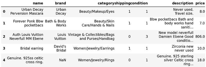
It consists of seven features including name, brand, and category of the product, who paid the shipping fee (the buyer or the seller), product condition and description, and the corresponding price in dollars. In building the model, the first six features are going to be your predictors and the price will be your target.

You will build your model step by step starting from the simplest and adding complexity along the way:

1. Baseline Model: from what humans would do to recommend a price
2. Machine Learning: classical models, made easy by PyCaret
3. Deep Learning: neural network models, leveraging TensorFlow

Baseline Model

In a real application, there are many tradeoffs to be considered when choosing a model. Besides performance, we should also consider how quickly the model responds for inference, time to retrain, computation cost, size in memory, interpretability, etc.

In terms of performance, the first thing we do is to build a simple baseline to compare the models. As this is a regression problem, we will consider simple metrics such as MAE, RMSE, and RMSLE for the performance.

First, we split the data with 12/1/1 proportion into train, validation, and test split. We won’t use the validation split to learn the hyperparameters for the moment since we don’t have any hyperparameters for this baseline model.

Train shape: (1200000, 7)
Validation shape: (100000, 7)
Test shape: (100000, 7)

For a baseline, we should consider the simplest yet sensible model. If your friend asks you, “How much does it cost?”, you would probably respond “What is ‘it’?”. A more appropriate question to be asked by your friend would be “How much does a phone cost?”, and hence you respond by “Hmm, about $800”.

Now, where does this $800 come from? A logical answer would be from a measure of the center of many phone prices, that is, from their mean or median (of course, the brand should be considered). Hence, to estimate a phone price, we group every phone and take the mean or median of their prices. We actually have this kind of group from our data: group by brand and by category.

name                0
brand          510245
category         4884
shipping            0
condition           0
description       657
price               0
dtype: int64

Since, from above, there are many missing values on brand, we'll use category instead. And since there are some particular phone brands that are significantly more expensive than others, the use of median aggregation is preferred.

There may be products where their category is newly introduced in the test split that has not been seen in the train split. In this case, the model can't predict the price of those products. We will handle this issue by simply imputing them by the median of all prices.

Here is the performance score of the baseline model.

Exploratory Data Analysis

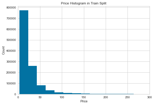
EDA should answer important questions and make it easier to extract insight. Here, our particular interest is about the price. Observing the histogram of price in train split, we directly see that its distribution follows Power Law where the relative change in one quantity varies as the power of another.

Some models such as those in the linear model family or neural network often perform better if the target variable follows a normal distribution. So, we may need to perform transformation for price, one of which is called box-cox transformation. Note that tree-based models are not affected by this.

See transformation in action below.

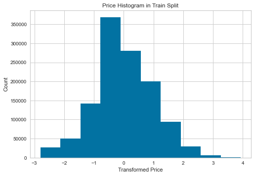
The resulted distribution is not necessarily normal, but it sure is more normal than the pre-transformed one.

Preprocessing

Before doing any modeling, we need to preprocess the data. For the preprocessing step, we do simple tasks as follows:

1. fill any missing value with an empty string,
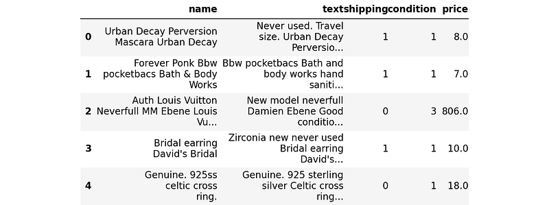
2. replace name by joining name and brand, separated by space,
3. make a new feature text by joining description, name, and category, separated by space,
4. drop all features except name, text, shipping, condition, and price (for target),
5. generate TF-IDF features from name and text, and
6. combine both TF-IDF features with text and shipping.

Below is the code, which is saved in a separate preprocess.py file in the working directory. This is important since later we use pickle implicitly and it needs the custom class(es) to be defined in another module/file and then imported. Otherwise, PicklingError will be raised.

As said before, import the necessary functions from preprocess.py. Note that we also import gc as a garbage collector to release memory when the object is no longer in use (since our data is big).

Now, preprocess the data.

Machine Learning

As an intern, suppose you don’t know deeply about the art and craft of machine learning algorithms. You need a low-code machine learning library to help you do most of the work.

Behold, PyCaret.

What we do in this section is inspired by a PyCaret tutorial. Shoutout to Moez Ali and team, we couldn’t thank you enough 👏.

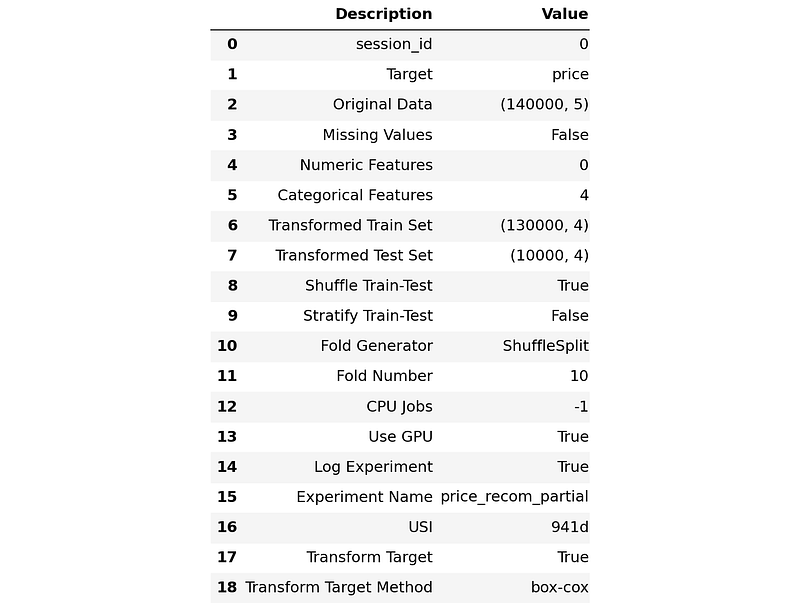
Create a TF-IDF vectorizer. For now, we will use max_features = 10000, but will be increased later on. We build an experiment setup with several keynotes:

1. data used is only 0.1 of all observations for first prototyping, chosen randomly,
2. no further preprocessing is done on predictors,
3. the price is transformed by box-cox transformation as suggested by EDA, and
4. the training strategy is simply by splitting the train split into train and validation split.

We could see the available models from PyCaret by calling the models function.

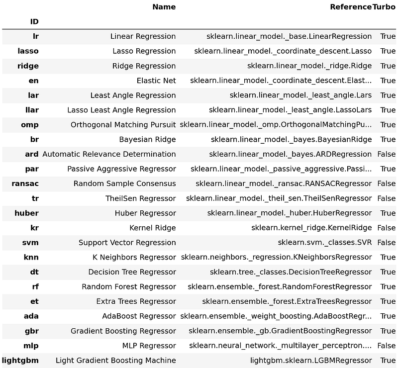
Next, pick some models and compare them. Here we choose eight of them. You may want to try others.

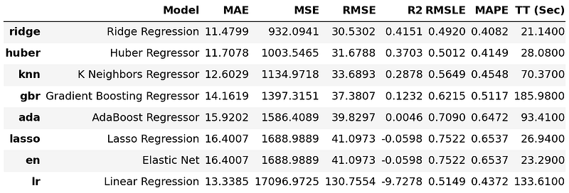
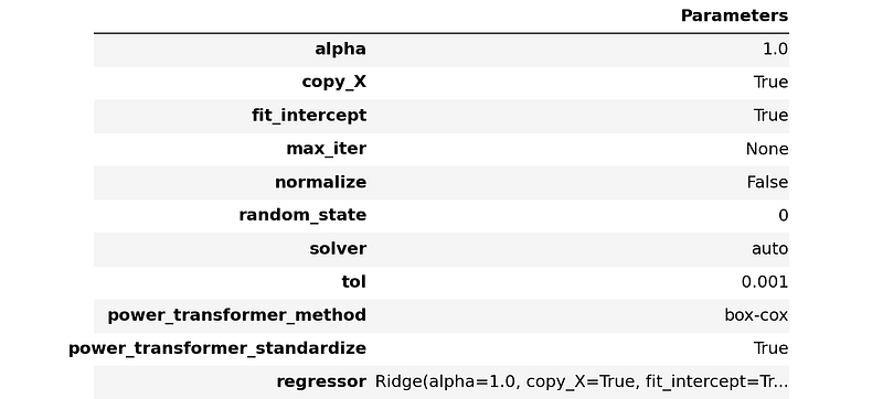
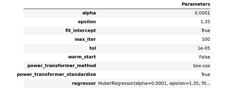
Some models perform better than the baseline model, some are worse. We can easily see that ridge and huber models perform really well indicated by their metrics, and their training time is among the fastest.

Delete some useless variables and free up some memory.

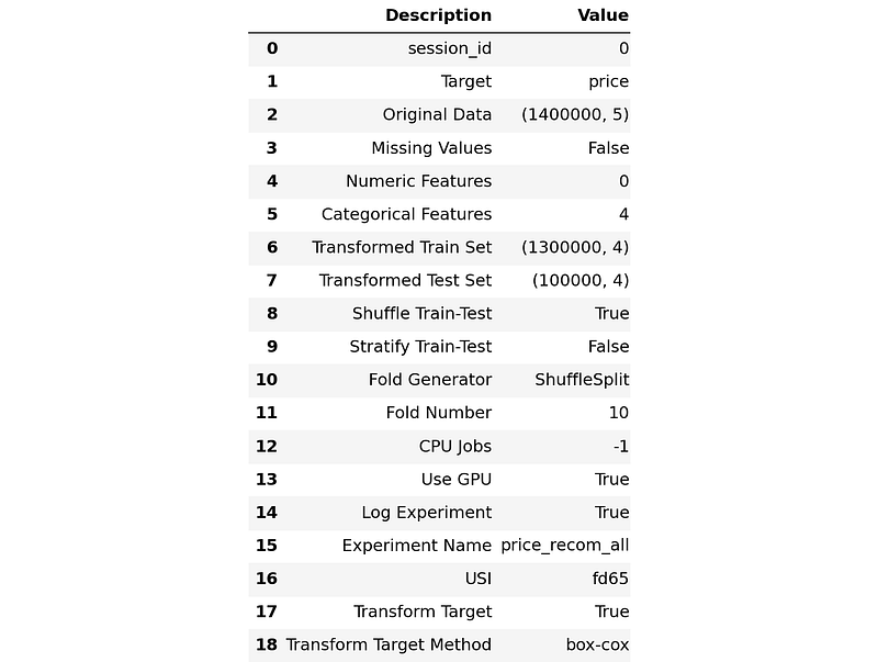
146

Now, create another TF-IDF vectorizer with max_features = 100000. The new experiment setup is the same as before except for now we use the new vectorizer and all observations in the data.

With this new setup, we train the two best performing models, ridge and huber. We can see that there is an increment in the performance.

We can also blend both models.

The blended model is definitely better than huber. Also, the blended model is slightly worse than ridge for all metrics except for RMSE where it wins significantly. We will choose the blended model as our champion (for the moment).

PyCaret is integrated with MLflow. You can start the MLflow UI to see the metadata of the current experiment on http://localhost:5000/ by running the command below in a terminal.

$ mlflow ui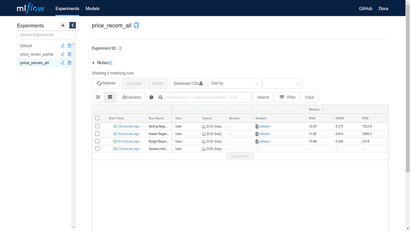

Let’s tabulate the result along with the baseline model.

There are many other features of PyCaret such as model tuning and other ensembling methods that we don’t explore here. You are encouraged to try those on your own tho.

Deep Learning

First, let’s vectorize the train and validation split as before.

X_train: (1200000, 193754) of float32
X_valid: (100000, 193754) of float32

Then, transform the price in validation split using the previously fitted box-cox transformation.

As mentioned above, we will use TensorFlow to aid us.

The simplest thing you can do in deep learning modeling is to build several layers of a dense neural network. Here, we build a network with three hidden layers that are trained for two epochs.

Let’s train two models from the X_train and X_valid pair.

Model 1
586/586 [========] - 11s 19ms/step - loss: 0.3623 - val_loss: 0.3151
293/293 [=========] - 8s 28ms/step - loss: 0.2163 - val_loss: 0.3077

Model 2
586/586 [========] - 11s 19ms/step - loss: 0.3626 - val_loss: 0.3178
293/293 [=========] - 8s 28ms/step - loss: 0.2171 - val_loss: 0.3078

Now, try something else by converting X_train and X_valid into boolean matrices, that is, if an element of X_train or X_valid is not zero then it’s changed to 1 and if an element is zero it stays 0. Train also two models with these new matrices.

Model 1
586/586 [========] - 11s 19ms/step - loss: 0.3682 - val_loss: 0.3247
293/293 [=========] - 8s 28ms/step - loss: 0.2103 - val_loss: 0.3151

Model 2
586/586 [========] - 12s 20ms/step - loss: 0.3680 - val_loss: 0.3250
293/293 [=========] - 8s 29ms/step - loss: 0.2101 - val_loss: 0.3162

Gather all four models into a python list and do predictions on all four validation splits. To be clear, these four models are:

1. Two models with TF-IDF data
2. Two models with boolean data

We build a score function to calculate the quality of the predictions.

For one model, we have the following score.

{'MAE': 9.2815766537261,
 'RMSE': 26.11544796731921,
 'RMSLE': 0.4090026031074859} 

By blending two models, we have the following score. There is a visible improvement.

{'MAE': 9.052237654724122,
 'RMSE': 25.90078324778221,
 'RMSLE': 0.4006770676979191} 

Lastly, the blend of all four models gives us the best result.

{'MAE': 8.918359263105392,
 'RMSE': 25.910815619338454,
 'RMSLE': 0.39423109095498304}

Append the result along with the baseline and machine learning one. We directly see that the deep learning model is the winner. Besides, the training time is also fast, less than 80 seconds.

Of course, we can further tune the hyperparameters of this model, or even try other neural network architectures. However, this article is getting too long to read. You are encouraged to try though.

Inference

Now, we will do predictions on the test split to confirm the final performance of our deep learning model. As before, the test split needs to be preprocessed before entering the model.

As expected, the score is similar to that of the validation split.

{'MAE': 8.916460799703598,
 'RMSE': 27.392445134423518,
 'RMSLE': 0.3933138510387536}

Finally, we save the model for future uses.

INFO:tensorflow:Assets written to: model1\assets
INFO:tensorflow:Assets written to: model2\assets
INFO:tensorflow:Assets written to: model3\assets
INFO:tensorflow:Assets written to: model4\assets

Conclusion

We’ve built a price recommendation system model for a case study of an e-commerce application. Starting with the baseline model, with minimum data preprocessing, we’ve achieved a pretty good result as follows.

We leveraged the use of PyCaret and TensorFlow to build the models. These libraries really do the hard work for us.

👏 Thanks! If you enjoy this story and want to support me as a writer, consider becoming a member. For only $5 a month, you’ll get unlimited access to all stories on Medium. If you sign up using my link, I’ll earn a small commission.

📧 If you’re one of my referred Medium members, feel free to email me at geoclid.members[at]gmail.com to get the complete python code of this story.

Prefer data science hands-on tutorials in R? Curious about how machine learning works? Check this out: