Coding

Predicting Stock Prices with Time Series Analysis in Python

Introduction to Prophet with examples

Stock prices exhibit trends and patterns, suggesting that a time series model could be instrumental in forecasting them.

Several general-purpose Python libraries offer capabilities for Time Series Analysis, including pycaret, statsmodels, and scikit-learn, among others. There are also libraries designed explicitly for Time Series Analysis, such as Prophet, Sktime, and Kats.

I opted to use Prophet for predicting stock prices because of its distinct focus on time series, user-friendly API, speedy performance (yielding results in seconds), and automation (eliminating the need for manual data processing).

Understanding Prophet

Developed by Meta, Prophet is an open-source library recognized for its rapid, fully automated forecasts that users can manually fine-tune.

Prophet employs an additive model to forecast time series data, accommodating non-linear trends with components for yearly, weekly, and daily seasonality, plus holiday impacts. This model excels with series demonstrating strong seasonal influences, benefiting from multiple historical data seasons. It manages missing data, trend changes, and outliers effectively.

Additive regression distinguishes itself as a flexible, non-parametric technique that doesn’t assume a fixed relationship model, which allows it to capture intricate, non-linear data dynamics, making it a potentially suitable model for stock market analyses.

Installing Prophet

To use Prophet, it must first be installed.

!pip install prophet

When working with Colab, I encountered an error that required the prior installation of pystan. To install pystan, execute:

!pip install pystan

Importing Libraries

In addition to Prophet, we’ll require yfinance for accessing stock data, pandas for data manipulation, plotly for visualization, and datetime for formatting data from yfinance for Prophet’s use.

Here is how to import these libraries:

import pandas as pd
from prophet import Prophet

import plotly.express as px
import plotly.io as pio
pio.renderers.default="colab"

import yfinance as yf
from datetime import datetime, timezone

Retrieving Stock Data

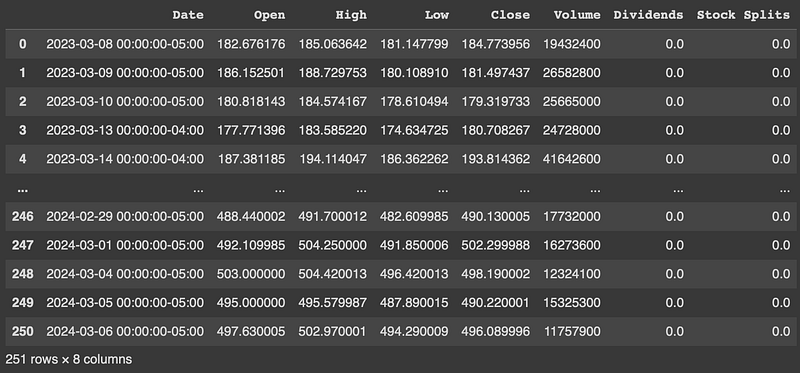
Taking META as an example, we retrieve its historical data as follows:

start_date_input = '2023-03-08'
end_date_input = '2024-03-07'

# Define the ticker symbol
tickerSymbol = 'META'

# Get data on this ticker
tickerData = yf.Ticker(tickerSymbol)

# Get the historical prices for this ticker
tickerDf = tickerData.history(period='1d', start=start_date_input, end=end_date_input)

# Make the index a column named "Date"
df = tickerDf.reset_index().rename(columns={"index":"Date"})

# Display the dataframe
display(df)

On successful execution, the dataframe should appear as follows:

Preparing Data for Prophet

Prophet expects a dataframe with two columns: ds and y.

We need to adapt the yfinance-derived dataframe accordingly.

columns = ["Date", "Close"]
ndf = pd.DataFrame(df, columns=columns)
# Prophet cannot use date with timezone.
ndf["Date"] = ndf["Date"].apply(lambda x: x.replace(tzinfo=None))

# Renaming Date to ds, Close to y.
prophet_df = ndf.rename(columns=({'Date':'ds', 'Close':'y'}))
display(prophet_df)

Forecasting with Prophet

First, we instantiate a new Prophet object. Then, we call its fit method by passing in the dataframe we have prepared for it.

After a quick model fitting, forecasting is achieved using Prophet’s make_future_dataframe method, which also includes historical date points by default.

m = Prophet()
m.fit(prophet_df)

future = m.make_future_dataframe(periods=30)
forecast_df = m.predict(future)
display(forecast_df)

The forecast display should resemble:

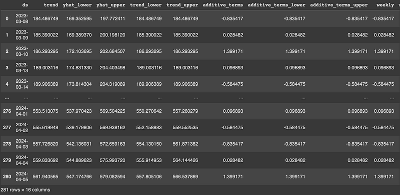
It comprises both historical and the next 30 days’ forecast data, with predicted values indicated by yhat, including yhat_upper and yhat_lower confidence intervals.

Visualizing Results

Plotly express facilitates an intuitive visualization of the forecast data.

The forecast can be visualized via a single line of code:

px.line(forecast_df, x='ds', y='yhat')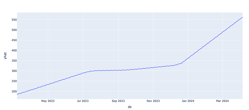

Prophet also provides a dedicated plotting function for detailed forecasting visualization.

figure = m.plot(forecast_df, xlabel='ds', ylabel='y')

This will show the prediction (yhat), the upper bound (yhat_upper), the lower_bound (yhat_lower), and the historical stock values in the same graph:

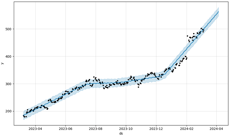
The graph shows data fluctuation around the yhat prediction.

Leveraging the Prediction

Although powerful, time series tools like Prophet cannot perfectly predict stock markets, which are subject to many influencing factors, including major events like earning calls, which can significantly impact trends beyond the predictive capability of time series models.

However, time series analysis can offer insightful predictions by sidelining major events.

For instance, leveraging a close enough prediction, could I place a cover call slightly above the upper prediction boundary to earn extra income without stock sale risk?

On March 8th, I sold to open a META call at a strike price of 570 set for expiration on March 22nd, yielding $234.34. Prophet’s upper bound prediction was $549.35. So, I have a $20 safety buffer.

Let’s see how this investment strategy unfolds with Prophet’s insights. Wish me luck!

Hi, I am Cat. I am a writer, artist, and snowboarder disguised as a software engineer during the day. I’d love you to follow me (Cat S Guan) to see my stories on your feed. To have stories sent directly to you, subscribe to my newsletter. 👇

A Message from InsiderFinance

Thanks for being a part of our community! Before you go:

• 👏 Clap for the story and follow the author 👉
• 📰 View more content in the InsiderFinance Wire
• 📚 Take our FREE Masterclass
• 📈 Discover Powerful Trading Tools