Predicting Results and Goals with Machine Learning

I have created a model to predict the outcome of the FIFA World Cup games

We are now one week deep into the FIFA World Cup 2022. More than 20 games have already occurred with some pretty “predictable” results, as well as some surprises, what is somewhat not uncommon in football (or soccer, whatever you want to call it).

A couple of days before the championship’s kick off, I started to see some posts with these nice models from other data scientists trying to predict the outcome of the games and, of course, predict the champion. After all, the World Cup is one of the most desired trophies in this sport.

For me, as a football lover (I am Brazilian, I call it football because the game is played with the feet… :-) ), I got double interested: (1) for the challenge of creating a model and practicing data science skills; (2) to work with such an interesting topic.

So, I went ahead and created a classification model to predict the result of the game (win, draw, lose). But I also wanted to be able to know the final score of the game, so I could play with my friends in those small betting competition to see who gets more results right. Therefore, I also created another model to predict that.

Also, let’s agree that football is a sport strongly reliant on the human factor, what makes it much more difficult to model. You will see that even with really good algorithms, the accuracy of the model is never too high. It is more like an informed guess, I’d say.

In this post, I will explain the approach I took for each step.

Let’s go.

Modeling the game result

The first part of the model was to predict the outcome of the game. Thus, I needed to create a classifier to predict one out of three classes: win, draw or lose. I know there are different ways to create such a model. You can use history of games, players data, coaches…

To me, while looking for World Cup historic data that could help me to model the problem, I bumped into this dataset from Kaggle [All the results from World Cups, under license CC0: Public Domain]. It is a dataset with all the games that have happened since the first World Cup in 1930. The data just didn’t have 2018’s edition. But that was easily inputted manually.

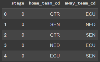
This way, I decided to move on modeling the problem based on results of the games from past World Cup editions. Here’s how the dataset looks like.

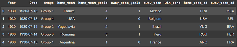
Ok, so we have dates, stage of the competition, home and away teams, goals and team codes. How to tell a machine learning model if that is either a win or lose, given every game has a winner AND a loser, right?

So I checked what’s the importance of the “home factor”, in other words, if the team playing as the home team wins or loses more. Figure 2 tells that story.

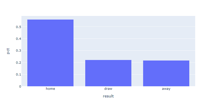
The higher bar for home team victories is explained by the way FIFA World Cup is constructed. The initial groups are composed by a head team (that is a strong team based on ranking) and other 3 that are between medium to weak. This is created to avoid group stage matches that could eliminate strong (commercially strong too) teams like Brazil, Germany, Argentina, Netherlands etc. As there are only 3 games by team in this first stage, the head of the group will be the home team in 2 games, and the away team 1. Therefore, with stronger teams playing at home, the number of victories increase.

Knowing all that, I decided to use the following classification labels: (-1) away team victory; (0) draw; (1) home team victory.

Next, I decided to make the first transformation to make the Group stage observations homogeneous. It won’t matter to my model if a team is either at group 1 or 4 or 6. It matters what’s the championship stage it is: groups.

# Wherever the stage variable does not have Group in the name, it stays the same. 
# Other cases, change to just "Group".
df['stage'] = df['stage'].where(~df.stage.str.contains('Group'), other='Group')

Where to find the pattern?

A machine learning model is a computer program that can take data in (usually numbers) and find patterns associated to labels.

So, if I find a pattern 1 associated to label A, every time it is found again, in whole or partially, by probability it is associated more or less with label A.

When creating this model, I thought about what could be the variables that would matter the most, other than the home and away factor. Since we’re dealing with historic games data, I thought that the model could compare the numbers of the home team against the away team’s number to create that pattern and predict the result. Thus, based on the initial dataset, these new variables were created: Games played, Wins at home, Wins away, Losses home, Losses away, Goals in favor [GF], Goals against [GA], Overall performance (victories/games played).

Since the a game is only played if there are two teams, naturally there will be a home and an away team. Let’s create variables for performance when a team is playing on each side. Next, we will create a dataset named teams_performance with the distinct teams from our data and start to join the variables for each indicator listed prior in this article.

Note: For Qatar, that never played any World Cup before, the numbers will be all zeroes.

The code is a little extense for a Medium post, but you can have access to the entire project in my GitHub.

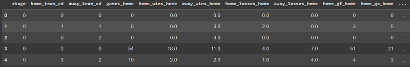
We will end up with this dataset.

# Teams Performance Dataset
teams_performance.sort_values(by='performance', ascending=False).head()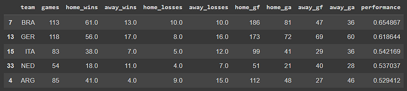

The Model

Ok, once the data was ready, I decided to make two more filters. The first one, I have separated the 2014 and 2018 editions to be the test set. The second one, I thought since football has changed so much in the last few years and sports technology also evolved so much, I decided to arbitrarily cut (and also based on trial and error) the training data for events after 1990, this last one not inclusive. So the World Cups considered for training were from 1994 to 2010. The test set was 2014 and 2018.

The input for the models was defined as these columns.

# X and y variables
X = train.drop(['home_team_goals','away_team_goals','result'], axis=1)
y = train.result

# Input variables
X.columns

Index(['stage', 'home_team_cd', 'away_team_cd', 'games_home', 'home_wins_home',
       'away_wins_home', 'home_losses_home', 'away_losses_home',
       'home_gf_home', 'home_ga_home', 'away_gf_home', 'away_ga_home',
       'performance_home', 'games_away', 'home_wins_away', 'away_wins_away',
       'home_losses_away', 'away_losses_away', 'home_gf_away', 'home_ga_away',
       'away_gf_away', 'away_ga_away', 'performance_away'],
      dtype='object')

Very well. First, I trained a CatBoost model and it did fairly good.

# Catboost
model = CatBoostClassifier(iterations=10000, learning_rate=0.55)
model.fit(X, y, cat_features= cat_features, verbose=2000)

0: learn: 0.9530572 total: 102ms remaining: 16m 55s
2000: learn: 0.0026780 total: 19.8s remaining: 1m 19s
4000: learn: 0.0012788 total: 31.2s remaining: 46.9s
6000: learn: 0.0008422 total: 41.7s remaining: 27.8s
8000: learn: 0.0006274 total: 52.2s remaining: 13s
9999: learn: 0.0005000 total: 1m 6s remaining: 0us
<catboost.core.CatBoostClassifier at 0x7f84763a1890>

The error at the end of the training error was small and the F1 score was nice too.

pred_train = model.predict(X) 
pred_test = model.predict(Xt)
# Test Score
f1_score(yt, pred_test, average=None)

array([0.6122449 , 0.24561404, 0.69172932])

Here is the confusion matrix for the test set.

# Confusion Matrix Test
pd.DataFrame(confusion_matrix(y_true=yt, y_pred=pred_test), 
             index=['away', 'draw', 'home'],
             columns=['away', 'draw', 'home'])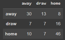

The second model trained was a Random Forest [RF]. I chose this model because of it’s robustness and versatility to solve complex problems. In addition, I had seen some good results from other people modeling this same kind of problem using RF.

But as RF required only numerical features, I had to create a function to change the variables stage, home_team_cd, away_team_cd to numeric.

# Function to factorize categorical features
def encode_variables(df):
  "Input a dataframe and return a dataframe whith categorical variables encoded numericaly"
  # Find categorical vars
  cat_vars = df.select_dtypes(include=['object', 'category']).columns
  # Loop and transform
  for variable in cat_vars:
    df[variable] = df[variable].factorize()[0]
  
  return df

# Encode categorical variables
X_rf = encode_variables(X_rf)

# Encode categorical variables
Xt_rf = encode_variables(Xt_rf)

Moving on, I ran a dummy model to check the variables importances.

# Variable importances
x_scaled = StandardScaler().fit_transform(X_rf)
dummy = RandomForestClassifier().fit(x_scaled, y)
dummy_importances = pd.DataFrame({'variables':X_rf.columns,
                                  'importance': dummy.feature_importances_}).sort_values(by='importance', ascending=False)
px.bar(dummy_importances,
       x= 'variables', y='importance',
       height=500, width=1000)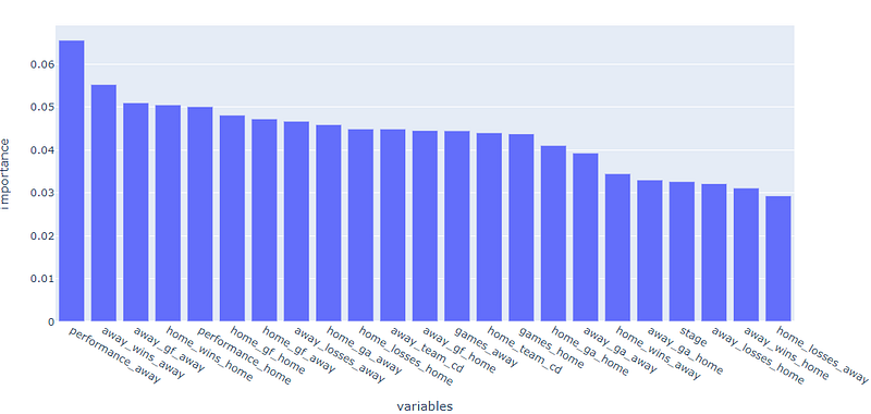

See that, besides performance_away , the other variables are pretty much alike until the last six or so that will fall under 4%. Seeing this, I decided to move on with all the variables.

I also scaled the variables, since I didn’t want the model to differentiate too much numbers in different scales, like Goals and number of games from other variables. So, instead of performing the standardization and then modeling, we can create a shortcut with a pipeline. This object scales the data, fit the model and can be used for predictions.

# Steps
steps = [
    ('scale', StandardScaler()),
    ('model', RandomForestClassifier())
]

# Final Pipeline
model_rf = Pipeline( steps )
# Fit
model_rf.fit(X_rf, y)

# Model predictions
pred_rf_test = model_rf.predict(Xt_rf)

Let’s take a look at the results.

# Test confusion matrix
pd.DataFrame(confusion_matrix(y_true=yt, y_pred=pred_rf_test), 
             index=['away', 'draw', 'home'],
             columns=['away', 'draw', 'home'])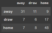

# F1 score
f1_score(y_true=yt, y_pred=pred_rf_test, average=None)

array([0.64583333, 0.21818182, 0.70072993])

You can see that the results are very similar for each model. Therefore, I just moved forward with the RF model, given it is an algorithm that I had seen previous good results and that I could also use in ensembled with other models in a custom voting classifier in the next iteration, what we will see next.

Voting Classifier

I tried to improve the model by creating a custom voting classifier composed of two models: Logistic Regression and Random Forest.

# Models instances
logit = LogisticRegression(max_iter=10000, multi_class='multinomial')
rf = RandomForestClassifier(criterion='entropy', n_estimators=600, max_depth=3)
gb = GradientBoostingClassifier(learning_rate=0.3, n_estimators=10000)

# Voting Classifier
voting = VotingClassifier(estimators=[
          ('lr', logit),
          ('rf', rf) ],
           voting='soft')

# Fit
voting.fit(X_rf, y)

# F1 score
pred_voting = voting.predict(Xt_rf)
f1_score(y_true=yt, y_pred=pred_voting, average=None)

array([0.66      , 0.22222222, 0.74125874])

Slightly better than the previous two. Now let’s see them in practice!

Predictions

To put these models to work, I have created this file, also shared in GitHub for those who want to try.

From that, I merge the performance indicators created in the first part of this article and encoded the categorical variables.

# Let's create an input dataset for the model
X_input = (match
    .merge(teams_performance, left_on= 'home_team_cd', right_on='team', how='left').fillna(0)
    .merge(teams_performance, left_on= 'away_team_cd', right_on='team', suffixes=['_home','_away'], how='left').fillna(0) )
X_input.drop(['team_home', 'team_away'], axis=1, inplace=True)

X_input = encode_variables(X_input)

This is what we would see after the last code was executed.

After the model runs, the output will be the probabilities of winning, draw or losing of the home team. For example, for the opening game Qatar x Ecuador, the RF model gave this result: 44% for Ecuador winning. 41% for draw and 14% for Qatar.

# Results with Random Forest
model_rf.predict_proba(X_input)

#    prob_AWAY_TEAM, Draw, prob_HOME_TEAM
array([[0.44333333, 0.41  , 0.14666667])

Very nice! It actually got it right. The opening game ended Qatar 0 x 2 Ecuador!

But I wanted to go a little further and try to predict the scoreboard. How many goals each team will score? Let’s try to come up with a good guess next.

Modeling the number of goals

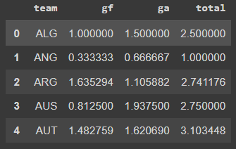
The first step of this modeling was to think about the inputs, once again. So I went back to the original dataset and created a table with the teams on the first column, the average of goals forward [gf], the goals against [ga] and total goals on average for each team.

Notice that the total can be interpreted as the total goals in a match. Think about it: the average of goals the team scored + the average it conceded is the match result.

# Goals Scored and Conceded
home_df = (df[['home_team_cd', 'home_team_goals', 'away_team_goals']]
           .rename(columns={'home_team_cd': 'team',
                            'home_team_goals': 'gf',
                            'away_team_goals':'ga'}) )
home_df['total'] = home_df.gf + home_df.ga

away_df = (df[['away_team_cd', 'home_team_goals', 'away_team_goals']]
           .rename(columns={'away_team_cd': 'team',
                            'home_team_goals': 'ga',
                            'away_team_goals':'gf'}) )
away_df['total'] = away_df.gf + away_df.ga

# Goals by team
df_goals = pd.concat([home_df, away_df], ignore_index=True)\
             .groupby('team').mean().reset_index()

Here’s how it looks like.

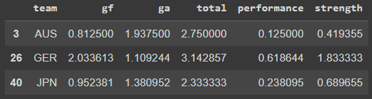
After that, I added the team’s historical performance (wins/games). And finally I came up with a strength indicator, that is [Goals in Favor]/[Goals Against]. This strength indicator will show me a percentage of the goals the team scores related to the goals it concedes. So the higher the number, the better is the attack and defense of that team, assuming that the division will be a high number of GF divided by a small number of GA.

Again, I have added some numbers for Qatar, as they do not hold World Cup history.

If we plot the total goals as a function of the other variables, we will see this.

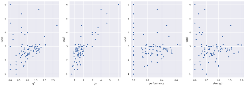
We can see that gf and ga hold some linear relationship with the total variable, that is what we will try to predict. ga has an 83% correlation. For gf, there are many points distorting the correlation and it is only 20%, but there’s still a pattern there.

So, I decided to try a linear model with SVR — from sklearn.svm import SVR. To force the model to consider a “match” between the team, the input will be the gf_home * ga_away and gf_away * ga_home, combined with the average of the performance numbers from both teams and the average of their strength numbers.

Simulating a match between Brazil x Italy.

# Data preparation for prediction of total goals in the match
my_input = df_goals.query('team in ["BRA", "ITA"]').drop(['team', 'total'], axis=1).reset_index(drop=True)
my_input.loc[len(my_input.index)] = [1.895, 1.58, 0.55, 1.82]

# Goal Linear Model
goal_model = SVR(C=1.0, kernel='poly', degree=1)
goal_model.fit(Xg, yg)

# Test prediction
goal_model.predict(my_input.iloc[2:,:])

array([3.52683536])

The average of goals expected is 3.52 goals.

To have an idea of performance, the model’s RMSE is at 1.8% off of the true mean.

# RMSE
rmse = np.sqrt( mean_squared_error( y_true=yg,
                            y_pred= goal_model.predict(Xg)) )
rmse

0.053057578470099995

# Variance of RMSE over the original mean
rmse / df_goals.total.mean()

0.018828

Awesome! Now we have a model to predict the match outcome and another one to predict the number of goals. We still need to make them work together to give us the final result.

Models working together

This will be done by a custom function (here in GitHub) that takes the names of the teams playing , the probabilities of the home team winning, the away team winning and draw. It will calculate the total goals in the match using the SVR model. Then, it multiplies the total by the winning probability of each team to determine the total of goals for each side.

Let’s says team A has 50% chance of winning and team B has 30%, with 20% chance of draw. If the total goals predicted was 4, team A gets 4*0.5 = 2 goals and team B gets 4*0.3=1.2 (1) goal. The result predicted will be team A 2x1 team B.

Predicting the Champion

Well… I created this model, like I said, to play with my friends and see how much I would be able to correctly predict using ML.

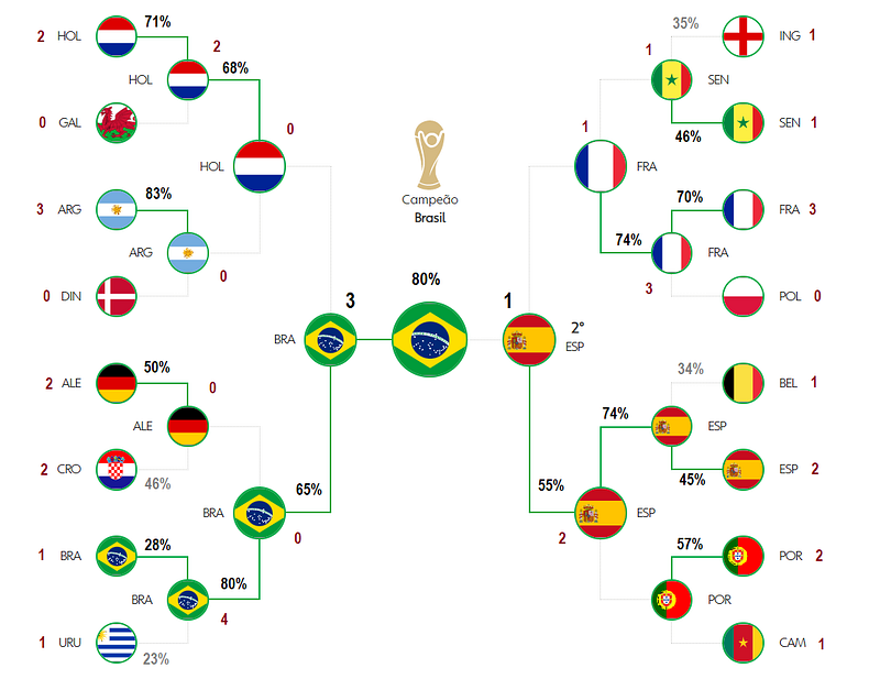
I ended up hitting the bull’s eye for some matches, like Senegal 0 x 2 Netherlands, or the USA 1 x 1 Wales. My model predicted France 5 x 0 Australia and the game ended on 4x1, fairly close.

So far, the Random Forest model is making 58% of correct predictions and the voting classifier is getting 45%. Those are nice numbers, given the complexity of predicting a something highly dependent on the human factor.

Regarding the champion, well, I hope my model is correct, because it is telling me Brazil is going to take this Cup home this year!

Will this model be accurate?

Time will tell.

Before You Go

We covered a lot in this article. Wow. Three models!

But I hope I could do that in a fun way for you to read, as much as it was fun to create them.

Here is the GitHub repository with all the code from this project, including datasets and results.

If you liked this content, follow my blog or find me in LinkedIn.

References