Practical Guide of Image Classification using CNN with Attention Mechanism

To display how to add attention layer, dropout layer and training the model with various callbacks for model checkpointing, learning rate reduction, and early stopping

Introduction

We have created a simple CNN model for image classification or recognition in the last article using the flower dataset as an example. This tutorial demonstrates the process of building, training, evaluating, and making predictions using a Convolutional Neural Network (CNN) with an attention mechanism for image recognition using the same flower dataset. The goal is to recognize different types of flowers based on images. The code uses the Keras/TensorFlow library for building and training the model, along with various callbacks for model checkpointing, learning rate reduction, and early stopping.

The process can be broken down into the following steps:

Data Preparation: The flower image dataset is split into training, validation, and test sets. Data augmentation techniques are applied to the training set to increase its size and improve model generalization.
Model Creation: The CNN model is designed with convolutional layers, pooling layers, dropout layers for regularization, and an attention mechanism to emphasize relevant image regions. The model is compiled with the categorical crossentropy loss function and the Adam optimizer.
Model Training: The model is trained on the training set using the fit method. Callbacks are utilized to save the best model based on validation accuracy, reduce the learning rate when validation loss plateaus, and stop training early if validation accuracy does not improve.
Model Evaluation: The trained model is evaluated on the test set to assess its performance on unseen data. The test loss and test accuracy are computed to quantify its effectiveness in flower recognition.
Prediction and Visualization: The model is used to make predictions on a few sample images from the test set. The true and predicted labels are displayed alongside the sample images to visualize the model’s performance.

Let’s dive into the implementation step by step. Before starting the process, please make sure that you have installed all the libraries imported in the step 1.

· Introduction · Brief Explaination of Attention · Step 1: Import libraries · Step 2: Data Preparation and Generators · Step 3: Display Sample Images from the Training Set · Step 4: Creating a CNN Model with Attention Mechanism · Step 5: Display the summary and the architecture of the model · Step 6: Define Model Callbacks · Step 7: Train the model and save the best model based on validation accuracy · Step 8: Plot Training and Validation Metrics · Step 9: Predicting on the Test Set and Displaying Results · Step 10: Evaluate the model on the test set · Conclusion

Brief Explaination of Attention

Attention is a mechanism in deep learning that allows a model to focus on specific parts of input data while making predictions or decisions. The idea of attention is inspired by human cognitive processes, where we tend to selectively pay attention to relevant information while ignoring irrelevant details. In the context of neural networks, attention mechanisms help improve the model’s ability to process long sequences or large inputs effectively.

In natural language processing (NLP) tasks, such as machine translation or text summarization, attention mechanisms are widely used to highlight relevant words or phrases in the input text when generating the output. This enables the model to focus on the most critical parts of the text and align the context between input and output sequences effectively.

In computer vision tasks, attention mechanisms have been employed in various architectures, especially in tasks that require processing images or long sequences of data. For example, in image captioning, the attention mechanism allows the model to focus on specific regions of the image when generating captions, ensuring that the generated description aligns well with the salient objects or regions in the image.

One common type of attention mechanism is called “soft attention” or “soft attention weighting.” In this approach, the attention mechanism generates a weight or attention score for each element in the input sequence or image, indicating its relevance or importance. These attention weights are then used to compute a weighted sum of the input elements, where elements with higher attention scores contribute more to the final prediction or output.

Attention mechanisms have proven to be effective in various tasks, providing better interpretability, reducing computational complexity, and improving model performance by allowing the model to focus on the most informative parts of the input data. They have become an essential tool in modern deep learning models, particularly in tasks involving sequential data, image analysis, and natural language processing.

Step 1: Import libraries

let’s import various Python libraries that are required for the whole tutorial.

import numpy as np
import os
import matplotlib.pyplot as plt
from keras.models import Model
from keras.layers import Input, Conv2D, MaxPooling2D, Flatten, Dense, GlobalAveragePooling2D, multiply, Dropout
from keras.preprocessing.image import ImageDataGenerator
from keras.callbacks import ModelCheckpoint, ReduceLROnPlateau, EarlyStopping
from PIL import Image

Step 2: Data Preparation and Generators

This step will set up data generators that will be used to feed image data to the model during training, validation, and testing. The training data generator applies data augmentation techniques to enhance the model’s ability to generalize, while the validation and test data generators only rescale the pixel values without augmentation.

# Set the path to the dataset folder
data_path = "./flowers_split_data"

# Create data generators for training and test
train_datagen = ImageDataGenerator(rescale=1./255, shear_range=0.2, zoom_range=0.2, horizontal_flip=True)

val_datagen = ImageDataGenerator(rescale=1./255) 
test_datagen = ImageDataGenerator(rescale=1./255)

train_generator = train_datagen.flow_from_directory(
    os.path.join(data_path, "train"),
    target_size=(128, 128),
    batch_size=32,
    class_mode='categorical'
)

val_generator = val_datagen.flow_from_directory(
    os.path.join(data_path, "val"),
    target_size=(128, 128),
    batch_size=32,
    class_mode='categorical'
)  

# Test the model on a few samples
test_generator = val_datagen.flow_from_directory(
    os.path.join(data_path, "test"),
    target_size=(128, 128),
    batch_size=32,
    class_mode='categorical', 
    shuffle=False
)

Found 3019 images belonging to 5 classes.
Found 644 images belonging to 5 classes.
Found 654 images belonging to 5 classes.

These messages provide information about the number of images and classes found in each dataset split. In details, the training data generator (‘train_generator’), the validation data generator (‘val_generator’), and the test data generator (‘test_generator’) have found 3019 images, 644 images and 654 images for training, validation and test, respectively, which belong to 5 different classes.

This messages confirms that the data generators have successfully discovered the dataset and are ready to provide batches of images during the model training and evaluation processes.

Step 3: Display Sample Images from the Training Set

In this step, we will display 6 sample images from the training set along with their filenames and training labels. It utilizes the train_generator previously defined to fetch the images and their corresponding labels.

# Get the class indices mapping (class labels to class names)
class_indices = train_generator.class_indices

# Display 6 sample images from the training set along with their filenames and training labels
plt.figure(figsize=(15, 12))
for i in range(6):
    img, label = train_generator.next()
    img_filename = train_generator.filenames[train_generator.batch_index - 1]  # Get the filename of the current image
    img_class = list(class_indices.keys())[list(class_indices.values()).index(label[0].argmax())]  # Get the class name
    plt.subplot(2, 3, i + 1)
    plt.imshow(img[0])
    plt.title(f"Image: {os.path.basename(img_filename)}\nLabel: {img_class}")
    plt.axis('off')

plt.tight_layout()
plt.show()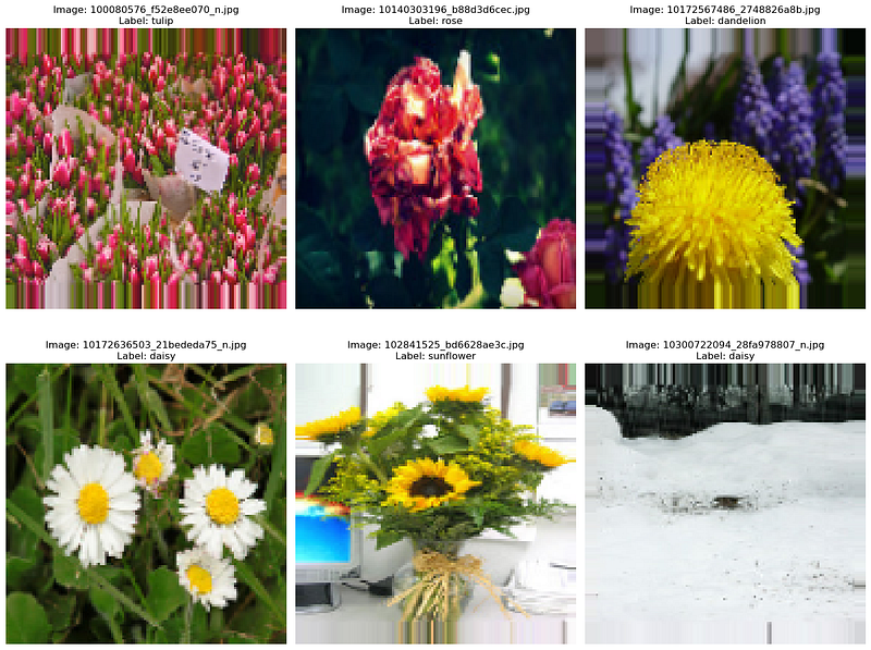

In this updated code, we access the train_generator.filenames attribute to retrieve the filenames of the current batch of images. We also use the train_generator.class_indices mapping to convert the label (one-hot encoded) to its corresponding class name. The argmax() function is used to find the index of the maximum value in the one-hot encoded label, which corresponds to the class with the highest probability.

The images are displayed along with their respective filenames and training labels (class names). The batch size of 32 is used in this example, so it may show the first 32 images from the training set. You can modify the code and loop as needed to display more images.

Step 4: Creating a CNN Model with Attention Mechanism

Next, we create a Convolutional Neural Network (CNN) model with an attention mechanism using Keras. The attention mechanism is introduced between the convolutional and pooling layers to highlight relevant features, which is usually used to emphasize certain parts of the input data during training, enabling the model to focus on relevant regions and improve its performance.

# Create a CNN model with attention mechanism
input_img = Input(shape=(128, 128, 3))
x = Conv2D(32, (3, 3), activation='relu')(input_img)
x = MaxPooling2D((2, 2))(x)
x = Dropout(0.1)(x)

# Add Attention Layer
attention = Conv2D(1, (1, 1), activation='sigmoid')(x)
x = multiply([x, attention])

x = Conv2D(64, (3, 3), activation='relu')(x)
x = MaxPooling2D((2, 2))(x)
x = Dropout(0.1)(x)

x = Conv2D(128, (3, 3), activation='relu')(x)
x = MaxPooling2D((2, 2))(x)
x = Dropout(0.25)(x)

x = Flatten()(x)
x = Dense(128, activation='relu')(x)
x = Dropout(0.5)(x)

output = Dense(5, activation='softmax')(x)  # 5 classes for flower recognition

model = Model(inputs=input_img, outputs=output)

# Compile the model
model.compile(optimizer='adam', loss='categorical_crossentropy', metrics=['accuracy'])

Step 5: Display the summary and the architecture of the model

The model.summary() method provides a concise summary of the architecture of the created CNN model, including the number of trainable parameters and the output shape of each layer. This summary allows you to quickly review the model's structure and the flow of data through its layers.

# Print the model summary
model.summary()

Model: "model"
__________________________________________________________________________________________________
 Layer (type)                Output Shape                 Param #   Connected to                  
==================================================================================================
 input_1 (InputLayer)        [(None, 128, 128, 3)]        0         []                            
                                                                                                  
 conv2d (Conv2D)             (None, 126, 126, 32)         896       ['input_1[0][0]']             
                                                                                                  
 max_pooling2d (MaxPooling2  (None, 63, 63, 32)           0         ['conv2d[0][0]']              
 D)                                                                                               
                                                                                                  
 dropout (Dropout)           (None, 63, 63, 32)           0         ['max_pooling2d[0][0]']       
                                                                                                  
 conv2d_1 (Conv2D)           (None, 63, 63, 1)            33        ['dropout[0][0]']             
                                                                                                  
 multiply (Multiply)         (None, 63, 63, 32)           0         ['dropout[0][0]',             
                                                                     'conv2d_1[0][0]']            
                                                                                                  
 conv2d_2 (Conv2D)           (None, 61, 61, 64)           18496     ['multiply[0][0]']            
                                                                                                  
 max_pooling2d_1 (MaxPoolin  (None, 30, 30, 64)           0         ['conv2d_2[0][0]']            
 g2D)                                                                                             
                                                                                                  
 dropout_1 (Dropout)         (None, 30, 30, 64)           0         ['max_pooling2d_1[0][0]']     
                                                                                                  
 conv2d_3 (Conv2D)           (None, 28, 28, 128)          73856     ['dropout_1[0][0]']           
                                                                                                  
 max_pooling2d_2 (MaxPoolin  (None, 14, 14, 128)          0         ['conv2d_3[0][0]']            
 g2D)                                                                                             
                                                                                                  
 dropout_2 (Dropout)         (None, 14, 14, 128)          0         ['max_pooling2d_2[0][0]']     
                                                                                                  
 flatten (Flatten)           (None, 25088)                0         ['dropout_2[0][0]']           
                                                                                                  
 dense (Dense)               (None, 128)                  3211392   ['flatten[0][0]']             
                                                                                                  
 dropout_3 (Dropout)         (None, 128)                  0         ['dense[0][0]']               
                                                                                                  
 dense_1 (Dense)             (None, 5)                    645       ['dropout_3[0][0]']           
                                                                                                  
==================================================================================================
Total params: 3305318 (12.61 MB)
Trainable params: 3305318 (12.61 MB)
Non-trainable params: 0 (0.00 Byte)
__________________________________________________________________________________________________

If you want to display the model architecture, you must install pydot (pip install pydot) and install graphviz for plot_model to work. You can refer to the previous CNN tutorial on the installation.

from keras.utils import plot_model

plot_model(model, to_file='model_architecture.png', show_shapes=True, show_layer_names=True)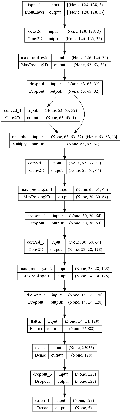

Step 6: Define Model Callbacks

In this section, you define three important callbacks to be used during the training process of the CNN model. Callbacks allow you to customize the training behavior and respond to certain events during the training, such as saving the best model, reducing learning rate, and early stopping.

# Define callbacks for model checkpoint, reduce learning rate and early stopping
checkpoint = ModelCheckpoint("./model/best_cnn_attention_flower.h5", 
                             monitor='val_accuracy', verbose=1, 
                             save_best_only=True, mode='max')
reduce_lr = ReduceLROnPlateau(monitor='val_accuracy', 
                              factor=0.2,
                              patience=5, 
                              min_lr=0)
early_stopping = EarlyStopping(monitor='val_accuracy', 
                               patience=15, verbose=1, 
                               restore_best_weights=True,
                               mode='max')

Step 7: Train the model and save the best model based on validation accuracy

In this section, the CNN model is trained using the fit method, and the previously defined callbacks (checkpoint, reduce_lr, and early_stopping) are used to customize the training process. Besides, we also use timeit.default_timer() function is used to measure the total training time in seconds.

import timeit
start_time = timeit.default_timer()
# Train the model
history = model.fit(
    train_generator,
    epochs=100,
    validation_data=val_generator, 
    callbacks=[checkpoint,reduce_lr,early_stopping]  # Use the checkpoint to save the best model
)
elapsed = timeit.default_timer() - start_time 
print("Total time: ", elapsed, "seconds")

Epoch 1/100
95/95 [==============================] - ETA: 0s - loss: 1.4142 - accuracy: 0.3620
Epoch 1: val_accuracy improved from -inf to 0.51242, saving model to ./model\best_cnn_attention_flower.h5
95/95 [==============================] - 59s 598ms/step - loss: 1.4142 - accuracy: 0.3620 - val_loss: 1.1843 - val_accuracy: 0.5124 - lr: 0.0010
Epoch 2/100


C:\ProgramData\anaconda3\Lib\site-packages\keras\src\engine\training.py:3000: UserWarning: You are saving your model as an HDF5 file via `model.save()`. This file format is considered legacy. We recommend using instead the native Keras format, e.g. `model.save('my_model.keras')`.
  saving_api.save_model(


95/95 [==============================] - ETA: 0s - loss: 1.1643 - accuracy: 0.5035
Epoch 2: val_accuracy improved from 0.51242 to 0.56056, saving model to ./model\best_cnn_attention_flower.h5
95/95 [==============================] - 56s 589ms/step - loss: 1.1643 - accuracy: 0.5035 - val_loss: 1.0895 - val_accuracy: 0.5606 - lr: 0.0010
Epoch 3/100
95/95 [==============================] - ETA: 0s - loss: 1.0818 - accuracy: 0.5518
Epoch 3: val_accuracy improved from 0.56056 to 0.57298, saving model to ./model\best_cnn_attention_flower.h5
95/95 [==============================] - 56s 585ms/step - loss: 1.0818 - accuracy: 0.5518 - val_loss: 1.0540 - val_accuracy: 0.5730 - lr: 0.0010
Epoch 4/100
95/95 [==============================] - ETA: 0s - loss: 1.0141 - accuracy: 0.5972
Epoch 4: val_accuracy improved from 0.57298 to 0.58540, saving model to ./model\best_cnn_attention_flower.h5
95/95 [==============================] - 57s 600ms/step - loss: 1.0141 - accuracy: 0.5972 - val_loss: 0.9912 - val_accuracy: 0.5854 - lr: 0.0010
Epoch 5/100
95/95 [==============================] - ETA: 0s - loss: 0.9495 - accuracy: 0.6300
Epoch 5: val_accuracy improved from 0.58540 to 0.63199, saving model to ./model\best_cnn_attention_flower.h5
95/95 [==============================] - 56s 590ms/step - loss: 0.9495 - accuracy: 0.6300 - val_loss: 0.9181 - val_accuracy: 0.6320 - lr: 0.0010
Epoch 6/100
95/95 [==============================] - ETA: 0s - loss: 0.9056 - accuracy: 0.6611
Epoch 6: val_accuracy improved from 0.63199 to 0.64441, saving model to ./model\best_cnn_attention_flower.h5
95/95 [==============================] - 57s 597ms/step - loss: 0.9056 - accuracy: 0.6611 - val_loss: 0.9262 - val_accuracy: 0.6444 - lr: 0.0010
Epoch 7/100
95/95 [==============================] - ETA: 0s - loss: 0.8646 - accuracy: 0.6618
Epoch 7: val_accuracy improved from 0.64441 to 0.65839, saving model to ./model\best_cnn_attention_flower.h5
95/95 [==============================] - 57s 594ms/step - loss: 0.8646 - accuracy: 0.6618 - val_loss: 0.8700 - val_accuracy: 0.6584 - lr: 0.0010
Epoch 8/100
95/95 [==============================] - ETA: 0s - loss: 0.8253 - accuracy: 0.6843
Epoch 8: val_accuracy did not improve from 0.65839
95/95 [==============================] - 56s 590ms/step - loss: 0.8253 - accuracy: 0.6843 - val_loss: 0.8942 - val_accuracy: 0.6553 - lr: 0.0010
Epoch 9/100
95/95 [==============================] - ETA: 0s - loss: 0.8059 - accuracy: 0.6906
Epoch 9: val_accuracy improved from 0.65839 to 0.67702, saving model to ./model\best_cnn_attention_flower.h5
95/95 [==============================] - 57s 594ms/step - loss: 0.8059 - accuracy: 0.6906 - val_loss: 0.8645 - val_accuracy: 0.6770 - lr: 0.0010
Epoch 10/100
95/95 [==============================] - ETA: 0s - loss: 0.7616 - accuracy: 0.7184
Epoch 10: val_accuracy improved from 0.67702 to 0.68789, saving model to ./model\best_cnn_attention_flower.h5
95/95 [==============================] - 56s 591ms/step - loss: 0.7616 - accuracy: 0.7184 - val_loss: 0.8542 - val_accuracy: 0.6879 - lr: 0.0010
Epoch 11/100
95/95 [==============================] - ETA: 0s - loss: 0.7296 - accuracy: 0.7184
Epoch 11: val_accuracy did not improve from 0.68789
95/95 [==============================] - 56s 590ms/step - loss: 0.7296 - accuracy: 0.7184 - val_loss: 0.8336 - val_accuracy: 0.6786 - lr: 0.0010
Epoch 12/100
95/95 [==============================] - ETA: 0s - loss: 0.7108 - accuracy: 0.7271
Epoch 12: val_accuracy improved from 0.68789 to 0.69410, saving model to ./model\best_cnn_attention_flower.h5
95/95 [==============================] - 56s 586ms/step - loss: 0.7108 - accuracy: 0.7271 - val_loss: 0.8381 - val_accuracy: 0.6941 - lr: 0.0010
Epoch 13/100
95/95 [==============================] - ETA: 0s - loss: 0.6953 - accuracy: 0.7347
Epoch 13: val_accuracy did not improve from 0.69410
95/95 [==============================] - 56s 584ms/step - loss: 0.6953 - accuracy: 0.7347 - val_loss: 0.8374 - val_accuracy: 0.6848 - lr: 0.0010
Epoch 14/100
95/95 [==============================] - ETA: 0s - loss: 0.6590 - accuracy: 0.7493
Epoch 14: val_accuracy improved from 0.69410 to 0.70807, saving model to ./model\best_cnn_attention_flower.h5
95/95 [==============================] - 56s 591ms/step - loss: 0.6590 - accuracy: 0.7493 - val_loss: 0.8537 - val_accuracy: 0.7081 - lr: 0.0010
Epoch 15/100
95/95 [==============================] - ETA: 0s - loss: 0.6334 - accuracy: 0.7592
Epoch 15: val_accuracy did not improve from 0.70807
95/95 [==============================] - 55s 581ms/step - loss: 0.6334 - accuracy: 0.7592 - val_loss: 0.7851 - val_accuracy: 0.7065 - lr: 0.0010
Epoch 16/100
95/95 [==============================] - ETA: 0s - loss: 0.6210 - accuracy: 0.7642
Epoch 16: val_accuracy did not improve from 0.70807
95/95 [==============================] - 56s 586ms/step - loss: 0.6210 - accuracy: 0.7642 - val_loss: 0.8654 - val_accuracy: 0.6988 - lr: 0.0010
Epoch 17/100
95/95 [==============================] - ETA: 0s - loss: 0.6086 - accuracy: 0.7675
Epoch 17: val_accuracy did not improve from 0.70807
95/95 [==============================] - 55s 583ms/step - loss: 0.6086 - accuracy: 0.7675 - val_loss: 0.8733 - val_accuracy: 0.7003 - lr: 0.0010
Epoch 18/100
95/95 [==============================] - ETA: 0s - loss: 0.6038 - accuracy: 0.7767
Epoch 18: val_accuracy improved from 0.70807 to 0.71273, saving model to ./model\best_cnn_attention_flower.h5
95/95 [==============================] - 56s 589ms/step - loss: 0.6038 - accuracy: 0.7767 - val_loss: 0.8153 - val_accuracy: 0.7127 - lr: 0.0010
Epoch 19/100
95/95 [==============================] - ETA: 0s - loss: 0.5522 - accuracy: 0.7907
Epoch 19: val_accuracy did not improve from 0.71273
95/95 [==============================] - 56s 585ms/step - loss: 0.5522 - accuracy: 0.7907 - val_loss: 0.7863 - val_accuracy: 0.7050 - lr: 0.0010
Epoch 20/100
95/95 [==============================] - ETA: 0s - loss: 0.5302 - accuracy: 0.8032
Epoch 20: val_accuracy did not improve from 0.71273
95/95 [==============================] - 57s 599ms/step - loss: 0.5302 - accuracy: 0.8032 - val_loss: 0.8539 - val_accuracy: 0.7019 - lr: 0.0010
Epoch 21/100
95/95 [==============================] - ETA: 0s - loss: 0.5230 - accuracy: 0.8059
Epoch 21: val_accuracy did not improve from 0.71273
95/95 [==============================] - 56s 584ms/step - loss: 0.5230 - accuracy: 0.8059 - val_loss: 0.8225 - val_accuracy: 0.7065 - lr: 0.0010
Epoch 22/100
95/95 [==============================] - ETA: 0s - loss: 0.4786 - accuracy: 0.8178
Epoch 22: val_accuracy did not improve from 0.71273
95/95 [==============================] - 56s 585ms/step - loss: 0.4786 - accuracy: 0.8178 - val_loss: 0.9285 - val_accuracy: 0.6941 - lr: 0.0010
Epoch 23/100
95/95 [==============================] - ETA: 0s - loss: 0.4872 - accuracy: 0.8152
Epoch 23: val_accuracy improved from 0.71273 to 0.72826, saving model to ./model\best_cnn_attention_flower.h5
95/95 [==============================] - 56s 584ms/step - loss: 0.4872 - accuracy: 0.8152 - val_loss: 0.8524 - val_accuracy: 0.7283 - lr: 0.0010
Epoch 24/100
95/95 [==============================] - ETA: 0s - loss: 0.4556 - accuracy: 0.8208
Epoch 24: val_accuracy did not improve from 0.72826
95/95 [==============================] - 56s 586ms/step - loss: 0.4556 - accuracy: 0.8208 - val_loss: 0.8561 - val_accuracy: 0.7252 - lr: 0.0010
Epoch 25/100
95/95 [==============================] - ETA: 0s - loss: 0.4317 - accuracy: 0.8473
Epoch 25: val_accuracy did not improve from 0.72826
95/95 [==============================] - 57s 601ms/step - loss: 0.4317 - accuracy: 0.8473 - val_loss: 0.9593 - val_accuracy: 0.7081 - lr: 0.0010
Epoch 26/100
95/95 [==============================] - ETA: 0s - loss: 0.4196 - accuracy: 0.8374
Epoch 26: val_accuracy did not improve from 0.72826
95/95 [==============================] - 58s 605ms/step - loss: 0.4196 - accuracy: 0.8374 - val_loss: 0.8441 - val_accuracy: 0.7174 - lr: 0.0010
Epoch 27/100
95/95 [==============================] - ETA: 0s - loss: 0.4263 - accuracy: 0.8377
Epoch 27: val_accuracy did not improve from 0.72826
95/95 [==============================] - 58s 614ms/step - loss: 0.4263 - accuracy: 0.8377 - val_loss: 0.8585 - val_accuracy: 0.7112 - lr: 0.0010
Epoch 28/100
95/95 [==============================] - ETA: 0s - loss: 0.4139 - accuracy: 0.8460
Epoch 28: val_accuracy did not improve from 0.72826
95/95 [==============================] - 56s 592ms/step - loss: 0.4139 - accuracy: 0.8460 - val_loss: 0.9090 - val_accuracy: 0.7252 - lr: 0.0010
Epoch 29/100
95/95 [==============================] - ETA: 0s - loss: 0.3412 - accuracy: 0.8682
Epoch 29: val_accuracy improved from 0.72826 to 0.73913, saving model to ./model\best_cnn_attention_flower.h5
95/95 [==============================] - 58s 609ms/step - loss: 0.3412 - accuracy: 0.8682 - val_loss: 0.8620 - val_accuracy: 0.7391 - lr: 2.0000e-04
Epoch 30/100
95/95 [==============================] - ETA: 0s - loss: 0.3165 - accuracy: 0.8831
Epoch 30: val_accuracy improved from 0.73913 to 0.74224, saving model to ./model\best_cnn_attention_flower.h5
95/95 [==============================] - 56s 590ms/step - loss: 0.3165 - accuracy: 0.8831 - val_loss: 0.8908 - val_accuracy: 0.7422 - lr: 2.0000e-04
Epoch 31/100
95/95 [==============================] - ETA: 0s - loss: 0.3041 - accuracy: 0.8844
Epoch 31: val_accuracy did not improve from 0.74224
95/95 [==============================] - 61s 648ms/step - loss: 0.3041 - accuracy: 0.8844 - val_loss: 0.9234 - val_accuracy: 0.7314 - lr: 2.0000e-04
Epoch 32/100
95/95 [==============================] - ETA: 0s - loss: 0.2879 - accuracy: 0.8884
Epoch 32: val_accuracy improved from 0.74224 to 0.75000, saving model to ./model\best_cnn_attention_flower.h5
95/95 [==============================] - 61s 641ms/step - loss: 0.2879 - accuracy: 0.8884 - val_loss: 0.9062 - val_accuracy: 0.7500 - lr: 2.0000e-04
Epoch 33/100
95/95 [==============================] - ETA: 0s - loss: 0.2958 - accuracy: 0.8870
Epoch 33: val_accuracy improved from 0.75000 to 0.75311, saving model to ./model\best_cnn_attention_flower.h5
95/95 [==============================] - 55s 583ms/step - loss: 0.2958 - accuracy: 0.8870 - val_loss: 0.8923 - val_accuracy: 0.7531 - lr: 2.0000e-04
Epoch 34/100
95/95 [==============================] - ETA: 0s - loss: 0.2762 - accuracy: 0.8957
Epoch 34: val_accuracy did not improve from 0.75311
95/95 [==============================] - 55s 578ms/step - loss: 0.2762 - accuracy: 0.8957 - val_loss: 0.9258 - val_accuracy: 0.7469 - lr: 2.0000e-04
Epoch 35/100
95/95 [==============================] - ETA: 0s - loss: 0.2810 - accuracy: 0.8897
Epoch 35: val_accuracy did not improve from 0.75311
95/95 [==============================] - 57s 594ms/step - loss: 0.2810 - accuracy: 0.8897 - val_loss: 0.9108 - val_accuracy: 0.7469 - lr: 2.0000e-04
Epoch 36/100
95/95 [==============================] - ETA: 0s - loss: 0.2621 - accuracy: 0.8973
Epoch 36: val_accuracy improved from 0.75311 to 0.76398, saving model to ./model\best_cnn_attention_flower.h5
95/95 [==============================] - 56s 591ms/step - loss: 0.2621 - accuracy: 0.8973 - val_loss: 0.9370 - val_accuracy: 0.7640 - lr: 2.0000e-04
Epoch 37/100
95/95 [==============================] - ETA: 0s - loss: 0.2670 - accuracy: 0.8973
Epoch 37: val_accuracy did not improve from 0.76398
95/95 [==============================] - 55s 579ms/step - loss: 0.2670 - accuracy: 0.8973 - val_loss: 0.9525 - val_accuracy: 0.7578 - lr: 2.0000e-04
Epoch 38/100
95/95 [==============================] - ETA: 0s - loss: 0.2618 - accuracy: 0.8970
Epoch 38: val_accuracy did not improve from 0.76398
95/95 [==============================] - 64s 669ms/step - loss: 0.2618 - accuracy: 0.8970 - val_loss: 0.9380 - val_accuracy: 0.7609 - lr: 2.0000e-04
Epoch 39/100
95/95 [==============================] - ETA: 0s - loss: 0.2684 - accuracy: 0.8976
Epoch 39: val_accuracy did not improve from 0.76398
95/95 [==============================] - 60s 626ms/step - loss: 0.2684 - accuracy: 0.8976 - val_loss: 0.9820 - val_accuracy: 0.7422 - lr: 2.0000e-04
Epoch 40/100
95/95 [==============================] - ETA: 0s - loss: 0.2617 - accuracy: 0.9003
Epoch 40: val_accuracy did not improve from 0.76398
95/95 [==============================] - 55s 577ms/step - loss: 0.2617 - accuracy: 0.9003 - val_loss: 0.9806 - val_accuracy: 0.7593 - lr: 2.0000e-04
Epoch 41/100
95/95 [==============================] - ETA: 0s - loss: 0.2369 - accuracy: 0.9063
Epoch 41: val_accuracy did not improve from 0.76398
95/95 [==============================] - 55s 581ms/step - loss: 0.2369 - accuracy: 0.9063 - val_loss: 0.9852 - val_accuracy: 0.7624 - lr: 2.0000e-04
Epoch 42/100
95/95 [==============================] - ETA: 0s - loss: 0.2263 - accuracy: 0.9149
Epoch 42: val_accuracy did not improve from 0.76398
95/95 [==============================] - 57s 602ms/step - loss: 0.2263 - accuracy: 0.9149 - val_loss: 0.9856 - val_accuracy: 0.7593 - lr: 4.0000e-05
Epoch 43/100
95/95 [==============================] - ETA: 0s - loss: 0.2384 - accuracy: 0.9149
Epoch 43: val_accuracy did not improve from 0.76398
95/95 [==============================] - 58s 603ms/step - loss: 0.2384 - accuracy: 0.9149 - val_loss: 0.9800 - val_accuracy: 0.7593 - lr: 4.0000e-05
Epoch 44/100
95/95 [==============================] - ETA: 0s - loss: 0.2244 - accuracy: 0.9142
Epoch 44: val_accuracy did not improve from 0.76398
95/95 [==============================] - 57s 600ms/step - loss: 0.2244 - accuracy: 0.9142 - val_loss: 0.9801 - val_accuracy: 0.7578 - lr: 4.0000e-05
Epoch 45/100
95/95 [==============================] - ETA: 0s - loss: 0.2320 - accuracy: 0.9092
Epoch 45: val_accuracy did not improve from 0.76398
95/95 [==============================] - 56s 593ms/step - loss: 0.2320 - accuracy: 0.9092 - val_loss: 0.9833 - val_accuracy: 0.7516 - lr: 4.0000e-05
Epoch 46/100
95/95 [==============================] - ETA: 0s - loss: 0.2215 - accuracy: 0.9152
Epoch 46: val_accuracy did not improve from 0.76398
95/95 [==============================] - 56s 591ms/step - loss: 0.2215 - accuracy: 0.9152 - val_loss: 0.9870 - val_accuracy: 0.7484 - lr: 4.0000e-05
Epoch 47/100
95/95 [==============================] - ETA: 0s - loss: 0.2260 - accuracy: 0.9135
Epoch 47: val_accuracy did not improve from 0.76398
95/95 [==============================] - 56s 589ms/step - loss: 0.2260 - accuracy: 0.9135 - val_loss: 0.9797 - val_accuracy: 0.7562 - lr: 8.0000e-06
Epoch 48/100
95/95 [==============================] - ETA: 0s - loss: 0.2233 - accuracy: 0.9195
Epoch 48: val_accuracy did not improve from 0.76398
95/95 [==============================] - 56s 592ms/step - loss: 0.2233 - accuracy: 0.9195 - val_loss: 0.9804 - val_accuracy: 0.7578 - lr: 8.0000e-06
Epoch 49/100
95/95 [==============================] - ETA: 0s - loss: 0.2137 - accuracy: 0.9198
Epoch 49: val_accuracy did not improve from 0.76398
95/95 [==============================] - 56s 593ms/step - loss: 0.2137 - accuracy: 0.9198 - val_loss: 0.9818 - val_accuracy: 0.7547 - lr: 8.0000e-06
Epoch 50/100
95/95 [==============================] - ETA: 0s - loss: 0.2227 - accuracy: 0.9198
Epoch 50: val_accuracy did not improve from 0.76398
95/95 [==============================] - 57s 596ms/step - loss: 0.2227 - accuracy: 0.9198 - val_loss: 0.9862 - val_accuracy: 0.7562 - lr: 8.0000e-06
Epoch 51/100
95/95 [==============================] - ETA: 0s - loss: 0.2253 - accuracy: 0.9165
Epoch 51: val_accuracy did not improve from 0.76398
Restoring model weights from the end of the best epoch: 36.
95/95 [==============================] - 57s 601ms/step - loss: 0.2253 - accuracy: 0.9165 - val_loss: 0.9867 - val_accuracy: 0.7531 - lr: 8.0000e-06
Epoch 51: early stopping
Total time:  2893.630381199997 seconds

In summary, this code section trains the CNN model using the fit method and the specified callbacks. The model is trained for 100 epochs, and the callbacks help in saving the best model, reducing the learning rate, and early stopping based on the validation performance. The total training time is also measured and displayed at the end of the training process.

Step 8: Plot Training and Validation Metrics

Now, let’s plot the training and validation loss as well as the training and validation accuracy over the epochs of the model training. The history object, which was returned by the fit method during training, contains the training history, including the metrics computed during each epoch.

# Plot training and validation loss
plt.figure(figsize=(12, 6))
plt.subplot(1, 2, 1)
plt.plot(history.history['loss'], label='Training Loss')
plt.plot(history.history['val_loss'], label='Validation Loss')
plt.xlabel('Epoch')
plt.ylabel('Loss')
plt.legend()

# Plot training and validation accuracy
plt.subplot(1, 2, 2)
plt.plot(history.history['accuracy'], label='Training Accuracy')
plt.plot(history.history['val_accuracy'], label='Validation Accuracy')
plt.xlabel('Epoch')
plt.ylabel('Accuracy')
plt.legend()

plt.show()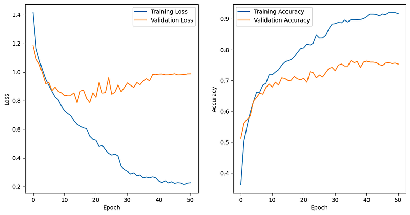

In summary, this code section plots two subplots side by side. The first subplot shows the training and validation loss over the epochs, and the second subplot shows the training and validation accuracy over the epochs. These plots provide valuable insights into the model’s training progress and its generalization performance on unseen data. The results show that the model is still overfitting although we add drop three dropout layers, and the main reason is that the training dataset is small. A small training dataset might not provide sufficient diverse examples to capture the full complexity of the flower recognition task. As a result, the model may memorize the training samples instead of learning generalized patterns, leading to poor generalization. to new data.

Step 9: Predicting on the Test Set and Displaying Results

In this section, the trained model is used to make predictions on the test set, and some sample images from the test set are displayed along with their true labels and predicted labels.

# Predict on the test set
predictions = model.predict(test_generator)

# Display some sample images from the test set along with their true and predicted labels
plt.figure(figsize=(15, 12))
for i in range(6):
    img, true_label = test_generator.next()
    img_filename = test_generator.filenames[test_generator.batch_index - 1]  # Get the filename of the current image
    true_class = list(test_generator.class_indices.keys())[list(test_generator.class_indices.values()).index(true_label.argmax())]  # Get the true class name
    predicted_class = list(test_generator.class_indices.keys())[list(test_generator.class_indices.values()).index(predictions[i].argmax())]  # Get the predicted class name

    plt.subplot(2, 3, i + 1)
    plt.imshow(img[0])
    plt.title(f"Image: {os.path.basename(img_filename)}\nTrue Label: {true_class}\nPredicted Label: {predicted_class}")
    plt.axis('off')

plt.tight_layout()
plt.show()

21/21 [==============================] - 7s 355ms/step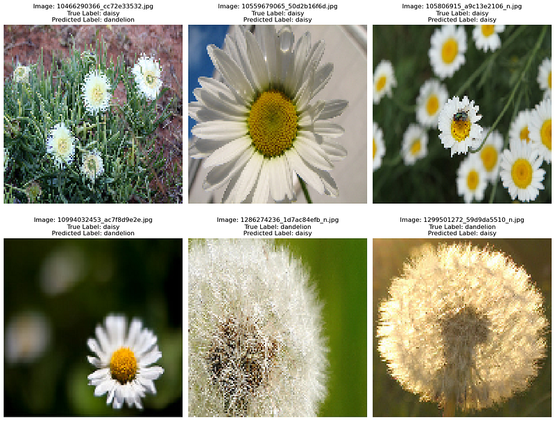

In summary, this step uses the trained model to predict the classes of some sample images from the test set and displays those images along with their true and predicted labels. It provides a visual evaluation of how well the model performs on unseen data.

Step 10: Evaluate the model on the test set

In this section, the trained model is evaluated on the entire test set to assess its performance on unseen data. The evaluation provides the test loss and test accuracy of the model.

# Evaluate the model on the test set
test_loss, test_accuracy = model.evaluate(test_generator)
print(f"Test Loss: {test_loss:.4f}")
print(f"Test Accuracy: {test_accuracy:.4f}")

21/21 [==============================] - 3s 131ms/step - loss: 0.7866 - accuracy: 0.7691
Test Loss: 0.7866
Test Accuracy: 0.7691

After loading trained model and the best weights using load_weights, we use evaluate to obtain the test loss and accuracy. These values are printed to the console. The evaluation results show that the prediction accuracy is only 76.91%.

Conclusion

The developed CNN model with an attention mechanism proves effective for flower recognition. By training on the provided dataset, the model achieves a satisfactory level of accuracy in distinguishing different types of flowers. Utilizing data augmentation and regularization techniques, the model exhibits generalization capabilities and avoids overfitting.

The attention mechanism incorporated into the model enhances its ability to focus on crucial image regions, leading to better performance. The use of model checkpoints, learning rate reduction, and early stopping through appropriate callbacks improves the training efficiency and prevents overfitting.

The results suggest that the model is still overfitting despite the inclusion of dropout layers. The primary reason attributed to this overfitting is the limited size of the training dataset, which hinders the model’s ability to learn generalized patterns effectively. The consequence of this limitation is that the model tends to memorize the training samples rather than capturing the full complexity of the flower recognition task, leading to poor generalization when applied to new and unseen data.

Furthermore, the results of another previous article highlights the potential benefits of employing a transfer learning approach to address the overfitting issue. Transfer learning involves leveraging knowledge learned from pre-trained models, typically trained on large and diverse datasets, and adapting it to the specific problem domain with limited data. By using transfer learning, the model can benefit from the rich representations learned from the large dataset, leading to improved validation and test accuracy.

In conclusion, the observations indicate that the small training dataset poses a significant challenge in achieving robust and generalized performance in the flower recognition task. Despite the inclusion of dropout layers, the model is still prone to overfitting. The suggestion of utilizing transfer learning from a pre-trained model presents a promising approach to mitigate the overfitting problem and enhance the model’s performance on validation and test data. The combination of data augmentation, regularization techniques, and transfer learning could potentially lead to a more robust and accurate flower recognition system.