Polynomial Regression: The Only Introduction You’ll Need

A deep-dive into the theory and application behind this Machine Learning algorithm in Python, by a student

Introduction

Polynomial Regression is, in my opinion, the natural second step in one’s progression through Machine Learning. Much more useful in the real world than Linear Regression, yet still easy to understand and implement.

As a student myself, I feel uniquely positioned to explain this concept to you, as I wish it was explained to me.

My goal here is to strike a balance between theory and implementation, leaving no stone unturned in my explanation of this algorithm’s inner workings, terminology, the mathematics upon which it is based and, finally, the code in which it is written, in a totally comprehensive yet beginner-friendly manner. One student to another.

So, welcome to the article I wish I could have read when I built my first Polynomial Regression model.

Important Note:

If you’re a beginner, I do recommend you read my article on Linear Regression first, which I’ve linked below. In it, I cover some foundational regression knowledge and terminology, upon which I will be building throughout this text, such as:

• A general introduction to regression analysis.
• An explanation of how regression works.
• Important terminology including R², Mean Squared Error and Variance.
• A detailed Linear Regression example.

If you are not familiar with anything I mentioned above, please read this article first, as I will not be explaining these concepts in detail again, and they are crucial.

The Theory

Polynomial Regression is a form of regression analysis in which the relationship between the independent variable x and the dependent variable y is modelled as an nth degree polynomial in x.

So what does that mean?

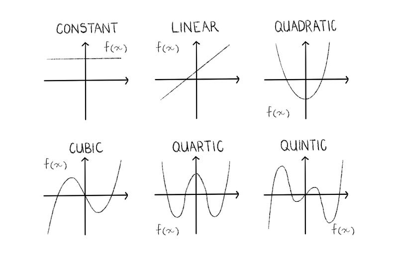
You may remember, from high school, the following functions:

Degree of 0 —> Constant function —> f(x) = a
Degree of 1 —> Linear function (straight line) —> f(x) = mx + c
Degree of 2 —> Quadratic function (parabola) —> f(x) = ax^2 + bx+ c
Degree of 3 —> Cubic function —> f(x) = ax^3 + bx^2 + cx + d

When writing a Polynomial Regression script, at some stage we must choose the degree to which we would like to plot our graph, as I shall demonstrate later. For now, let’s examine what this means for our function:

What is the degree?

Well, you may have noticed the pattern above: A polynomial’s degree is simply the highest power of any of its terms. So the degree we choose will dictate which function we fit to the data.

All of the above are polynomials.

Polynomial simply means “many terms” and is technically defined as an expression consisting of variables and coefficients, that involves only the operations of addition, subtraction, multiplication, and non-negative integer exponents of variables.

It’s worth noting that while linear functions do fit the definition of a polynomial in mathematics, in the context of Machine Learning, we can consider them to be two different methods of regression analysis.

Actually, Polynomial Regression is technically a type of Linear Regression. Although Polynomial Regression fits a nonlinear model to the data, as a statistical estimation problem it is linear, in the sense that the regression function E(y|x) is linear in the unknown parameters that are estimated from the data. Therefore, Polynomial Regression is considered to be a special case of Multiple Linear Regression.

In short: Think of Polynomial Regression as including quadratic and cubic functions, and Linear Regression as a linear function.

Terminology

Let’s quickly run through some important definitions:

Univariate / Bivariate

• A univariate dataset involves only one quantity, eg. times or weights, from which we can determine things like the mean, median, mode, range and standard deviation, and can be expressed as bar charts, pie charts and histograms.
• A bivariate dataset has two quantities, eg. sales over time, which we can use to compare data and find relationships, and can be expressed in scatter plots, correlation and regression.

Under-fitting / Over-fitting

• Under-fitting occurs when our statistical model cannot adequately capture the underlying structure of the data.
• Conversely, over-fitting produces an analysis that corresponds too closely to a particular set of data, and may therefore fail to fit additional data or predict future observations reliably.

The Algorithm

So, when would we choose Polynomial over Linear Regression?

There are 3 main situations that would warrant a Polynomial Regression over Linear:

1. The theoretical reason. The researcher (you) may hypothesise that the data will be curvilinear, in which case you should obviously fit it with a curve.
2. Upon a visual inspection of your data, a curvilinear relationship may be revealed. This could be achieved by a simple scatter plot (which is why you should always perform univariate and bivariate inspections of your data before applying a Regression Analysis).
3. Inspecting the model’s residuals. Attempting to fit a linear model to curvilinear data will result in high positive and negative residuals, and a low R² score.

Let’s go one step further. How do we choose the degree of our polynomial?

There are various mathematical analyses you can do to decide upon the best degree for your model, but it boils down to ensuring you aren’t under- or over-fitting the data. For our purposes, simply examining the scatter plot will reveal suitable options.

Remember that the way we perform regression analysis is by determining the coefficients that minimise the sum of the squared residuals.

The Example

First, the imports:

1. Pandas — To create a dataframe
2. Numpy — To do scientific computing
3. Matplotlib (pyplot and rcParams) — To create our data visualisations
4. Skikit-Learn (LinearRegression, train_test_split and PolynomialFeatures) — To perform Machine Learning

import pandas as pd
import matplotlib.pyplot as plt
from matplotlib import rcParams
from sklearn.model_selection import train_test_split
from sklearn.linear_model import LinearRegression
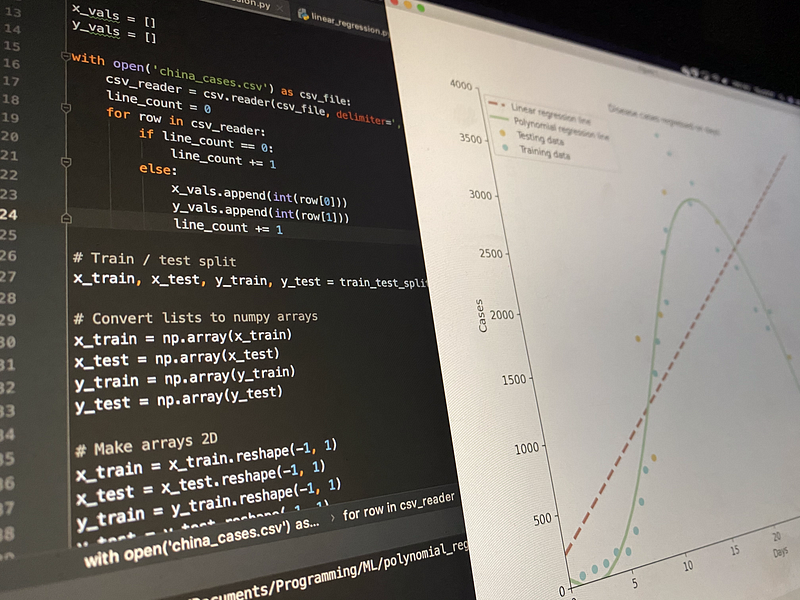
from sklearn.preprocessing import PolynomialFeatures

For this example I have created my own dataset, representing the amount of new COVID-19 cases recorded in China over 30 days, which I have stored in a csv file. The file looks like this:

x,y
1,59
2,77
3,93
...,...

Next, we use pandas to read the x an y values into two arrays. You could also do this with pandas’ iloc, or even without pandas at all, manually reading the data in from the file. This pandas method is just convenient as we can access the columns by name.

data = pd.read_csv('china_cases.csv')

x = data['x'].values
y = data['y'].values

We now have two arrays that look like this:

[1 2 3 4 5 ...]
[59 77 93 149 131 ...]

Let’s split our data into training and testing sets. We’ll use Skikit-Learn’s handy train_test_split function for this. We pass it the arrays of x and y values as arguments, in addition to a test size (how much of the data you want to be in the test portion) and a random state (an integer that dictates how the data is shuffled before being split. If you leave it out, your results will differ slightly each time you run the regression, so keep it in to reproduce your results, but you can remove it for production).

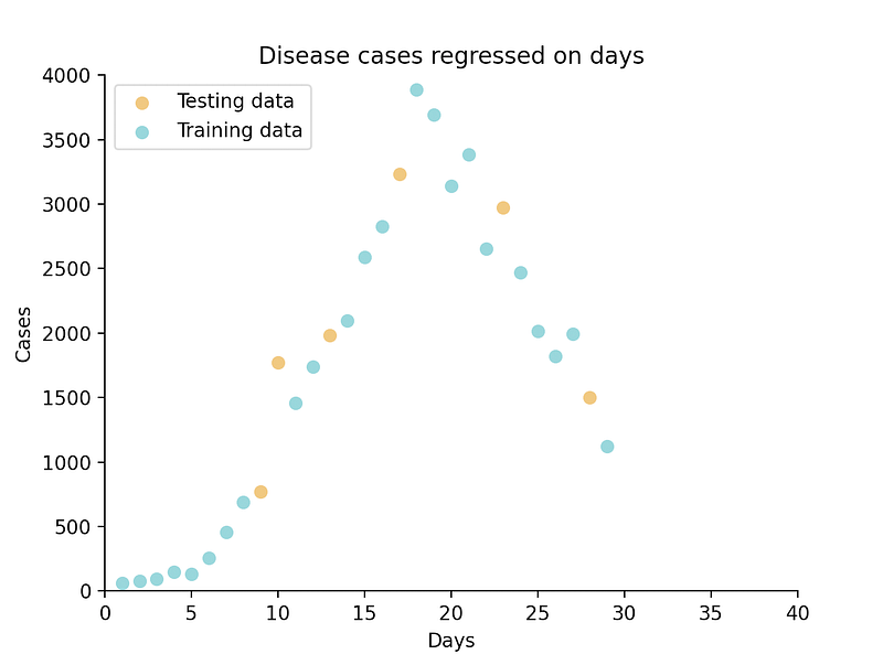
x_train, x_test, y_train, y_test = train_test_split(x, y, test_size=0.2, random_state=42)

Now is a good time to perform our bivariate inspection of the data, by means of a scatter plot. I’ll add some styling with rcParams and a legend to make it a little more visually appealing.

rcParams['axes.spines.top'] = False
rcParams['axes.spines.right'] = False

plt.scatter(x_test, y_test, c='#edbf6f', label='Testing data')
plt.scatter(x_train, y_train, c='#8acfd4', label='Training data')
plt.legend(loc="upper left")
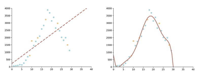
plt.show()

Below, you can clearly see that a linear model will not accurately fit this dataset, but it looks as though a quadratic or cubic function will work nicely.

At this point, we want to increase our arrays’ dimensionality to 2D, as this is the necessary matrix format required by the PolynomialFeatures class. We can achieve this simply by calling the reshape() function, where we define how we want our data to be shaped.

x_train = x_train.reshape(-1, 1)
y_train = y_train.reshape(-1, 1)

Our arrays now look something like this (this is x_train):

[[22]
 [ 1]
 [27]
 [14]
 [16]
  ...]

However, as you can see, the train_test_split shuffled our data, so it is no longer sorted. Matplotlib will plot the points in the order it receives them, so if we feed it our arrays as they are now, we’ll get some pretty weird results. To reorder the arrays, we sort y_train by x_train’s indices, and sort x_train itself.

y_train = y_train[x_train[:,0].argsort()]
x_train = x_train[x_train[:, 0].argsort()]

As I mentioned earlier, we have to set the degree of our polynomial. We do this by creating an object poly of the PolynomialFeatures class, and passing it our desired power as an argument.

poly = PolynomialFeatures(degree=2)

Additionally, we must transform our input data matrix into a new matrix of the given degree.

x_poly = poly.fit_transform(x_train)

All we have left to do is train our model. We create an object poly_reg of the LinearRegression class (remember that Polynomial Regression is technically linear, so it falls under the same class) and fit our transformed x values and y values to the model.

poly_reg = LinearRegression()
poly_reg.fit(x_poly, y_train)

Now we simply plot our line:

plt.title('Disease cases regressed on days')
plt.xlabel('Days')
plt.ylabel('Cases')
plt.plot(x_train, poly_reg.predict(x_poly), c='#a3cfa3', label='Polynomial regression line')
plt.legend(loc="upper left")
plt.show()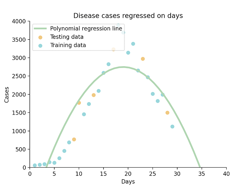

And there you have it, a quadratic function fitted to our data.

What if we set our degree to 3?

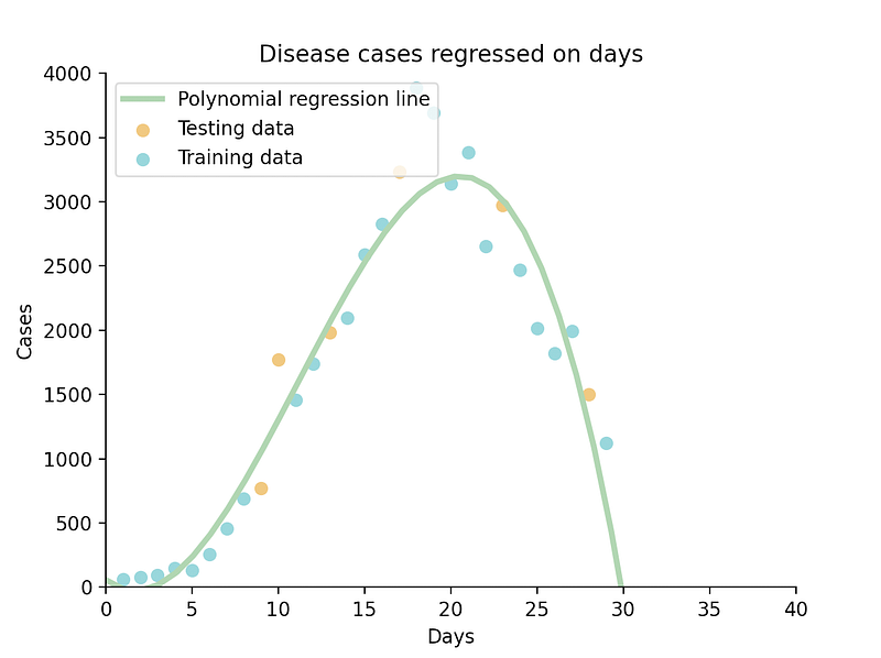
This cubic function seems to suit our data even better. Let’s examine their respective R² scores to get a clearer idea of their accuracy, by using the LinearRegression class’ .score() function:

print(poly_reg.score(x_poly, y_train))

Our quadratic function’s R² score is 0.81, while the cubic function’s is 0.93. In this case, I’d say the 3rd degree is a more suitable choice.

Note: if you choose 1 as the degree, you will perform a Linear Regression, but this would be a pretty round-about way of doing it.

If you’d like to read about another useful ML algorithm, K-Means, check this article out:

Conclusion

That concludes this thorough introduction to Machine Learning’s second simplest algorithm, Polynomial Regression. I hope that, as a student myself, I was able to explain the concepts relatably and comprehensively.

Let’s revise what we covered:

1. A reminder of what quadratic functions are.
2. Some important terminology.
3. An explanation of the algorithm, including when to use Polynomial Regression and how to choose the degree.
4. A practical example.
5. A comparison of using different degrees for our model.

If you found the article helpful, I’d love to engage with you! Follow me on Instagram for more Machine Learning, Software Engineering and Entrepreneurial content.

Happy coding!

Subscribe 📚 to never miss a new article of me, and if you aren’t a Medium member yet, join 🚀 to read all of my, and thousands of other stories!

Resources

The Analysis Factor Regression Models: https://www.theanalysisfactor.com/regression-modelshow-do-you-know-you-need-a-polynomial/

Wikipedia Overfitting: https://en.wikipedia.org/wiki/Overfitting

Math Is Fun Univariate and Bivariate Data: https://www.mathsisfun.com/data/univariate-bivariate.html

Stack Overflow Random State: https://stackoverflow.com/questions/28064634/random-state-pseudo-random-number-in-scikit-learn

Scikit-Learn sklearn.preprocessing.PolynomialFeatures: https://scikit-learn.org/stable/modules/generated/sklearn.preprocessing.PolynomialFeatures.html#sklearn.preprocessing.PolynomialFeatures.fit_transform

Scikit-Learn sklearn.linear_model.LinearRegression: https://scikit-learn.org/stable/modules/generated/sklearn.linear_model.LinearRegression.html

Scikit-Learn sklearn.model_selection.train_test_split: https://scikit-learn.org/stable/modules/generated/sklearn.model_selection.train_test_split.html

Stack Overflow Ordering Points: https://stackoverflow.com/questions/31653968/matplotlib-connecting-wrong-points-in-line-graph

Stack Overflow Sorting a list based on another list’s indices: https://stackoverflow.com/questions/6618515/sorting-list-based-on-values-from-another-list

Stack Overflow Sorting a 2D array by second column: https://stackoverflow.com/questions/22698687/how-to-sort-2d-array-numpy-ndarray-based-to-the-second-column-in-python