Plant Disease Classification with ResNet-9: Using PyTorch
Your Step-by-Step Guide to Saving Crops!
In this blog post, we’re diving into a practical and powerful project: building a Plant Disease Classifier using ResNet-9 in PyTorch. This guide is designed with beginners in mind, so if you’re new to PyTorch or Convolutional Neural Networks (CNNs), no worries — we’ll break down each step clearly. By the end, you’ll have a solid plant disease classifier ready to tackle real-world agricultural issues. 🌱

🌱 The Dataset: PlantVillage 🌱
We’ll use the PlantVillage dataset, which includes 87,000 RGB images of healthy and diseased leaves from various crops. These images are categorized into 38 different classes, representing different plants and diseases.
How We’ll Use It:
- 80/20 split for training and validation.
- A separate test directory with 33 images to check the model’s performance on unseen data.
Goal
We want our model to correctly identify whether a crop leaf is healthy or diseased. If diseased, it should predict the specific disease.
🚀 Let’s Get Started
1. Importing Libraries
First things first, let’s import the required libraries. If you haven’t installed torchsummary, go ahead and install it:
!pip install torchsummaryNow, let’s import the necessary modules:
import os
import numpy as np
import pandas as pd
import torch
import matplotlib.pyplot as plt
import torch.nn as nn
from torch.utils.data import DataLoader
from PIL import Image
import torch.nn.functional as F
import torchvision.transforms as transforms
from torchvision.utils import make_grid
from torchvision.datasets import ImageFolder
from torchsummary import summary
With these libraries, we can handle data, create neural networks, and apply image transformations.
Download link for the dataset
🧭 Exploring the Data
Now, let’s load the dataset and take a look at what we’re working with.
data_dir = "../input/new-plant-diseases-dataset/New Plant Diseases Dataset(Augmented)/New Plant Diseases Dataset(Augmented)"
train_dir = data_dir + "/train"
valid_dir = data_dir + "/valid"
diseases = os.listdir(train_dir)
print(diseases)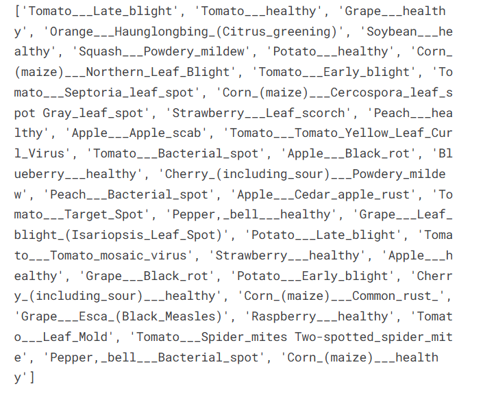
This will display the 38 classes in our dataset. To understand our dataset better, let’s count the unique plants and diseases.
plants = []
NumberOfDiseases = 0
for plant in diseases:
    if plant.split('___')[0] not in plants:
        plants.append(plant.split('___')[0])
    if plant.split('___')[1] != 'healthy':
        NumberOfDiseases += 1
In summary:
- 14 unique plants
- 26 unique diseases (excluding healthy classes)
📊 Visualizing Data Distribution
It’s always a good idea to understand the distribution of your data. Here, we’ll visualize the number of images per class.
nums = {}
for disease in diseases:
    nums[disease] = len(os.listdir(train_dir + '/' + disease))
img_per_class = pd.DataFrame(nums.values(), index=nums.keys(), columns=["no. of images"])
img_per_class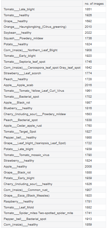
And let’s plot this:
plt.figure(figsize=(20, 5))
plt.bar([n for n in range(38)], [n for n in nums.values()], width=0.3)
plt.xlabel('Plants/Diseases', fontsize=10)
plt.ylabel('No of images available', fontsize=10)
plt.xticks([n for n in range(38)], diseases, fontsize=5, rotation=90)
plt.title('Images per each class of plant disease')
plt.show()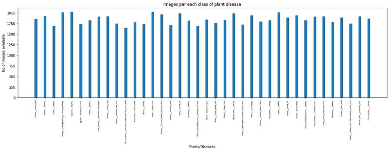
From the plot, we see that our dataset is fairly balanced across classes, which is excellent for training.
🍳 Data Preparation
To load our data, we’ll use PyTorch’s ImageFolder class, which organizes data based on folder structure.
train = ImageFolder(train_dir, transform=transforms.ToTensor())
valid = ImageFolder(valid_dir, transform=transforms.ToTensor())
Let’s check the shape of our images:
img, label = train[0]
print(img.shape, label)
Output:
torch.Size([3, 256, 256]) 0This shows our images are 256x256 RGB images.
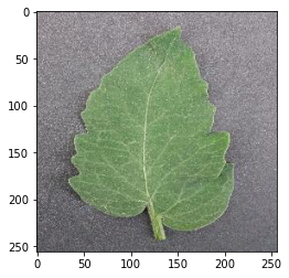
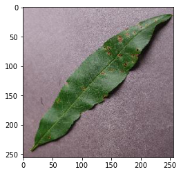
🖼️ Visualizing Sample Images
Let’s create a helper function to view some examples:
def show_image(image, label):
    print("Label :" + train.classes[label] + "(" + str(label) + ")")
    plt.imshow(image.permute(1, 2, 0))
Using this function:
show_image(*train[0])  # Example output: Apple___Apple_scab
show_image(*train[70000])  # Example output: Tomato___healthy
show_image(*train[30000])  # Example output: Peach___Bacterial_spot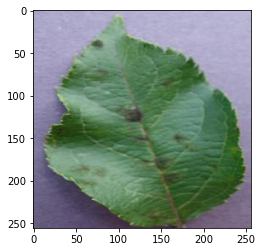
🏗️ Building the Model: ResNet-9
We’ll use a ResNet-9 architecture, a smaller but powerful CNN suitable for image classification. Before we define the model, let’s set up a few helper functions to manage the device.
Device Management
def get_default_device():
    return torch.device("cuda") if torch.cuda.is_available() else torch.device("cpu")
def to_device(data, device):
    if isinstance(data, (list, tuple)):
        return [to_device(x, device) for x in data]
    return data.to(device, non_blocking=True)
class DeviceDataLoader():
    def __init__(self, dl, device):
        self.dl = dl
        self.device = device

    def __iter__(self):
        for b in self.dl:
            yield to_device(b, self.device)

    def __len__(self):
        return len(self.dl)
Check the device:
device = get_default_device()
device
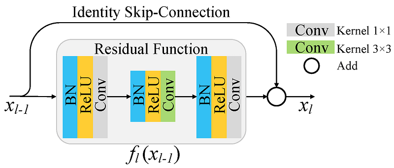
In ResNets, unlike in traditional neural networks, each layer feeds into the next layer, we use a network with residual blocks, each layer feeds into the next layer and directly into the layers about 2–3 hops away, to avoid over-fitting (a situation when validation loss stop decreasing at a point and then keeps increasing while training loss still decreases). This also helps in preventing vanishing gradient problem and allow us to train deep neural networks. Here is a simple residual block:
ResNet-9 Model Definition
Now, let’s define our model:
class ResNet9(nn.Module):
    def __init__(self, in_channels, num_classes):
        super().__init__()
        self.conv1 = self.ConvBlock(in_channels, 64)
        self.conv2 = self.ConvBlock(64, 128, pool=True)
        self.res1 = nn.Sequential(self.ConvBlock(128, 128), self.ConvBlock(128, 128))
        self.conv3 = self.ConvBlock(128, 256, pool=True)
        self.conv4 = self.ConvBlock(256, 512, pool=True)
        self.res2 = nn.Sequential(self.ConvBlock(512, 512), self.ConvBlock(512, 512))
        self.classifier = nn.Sequential(nn.MaxPool2d(4), nn.Flatten(), nn.Linear(512, num_classes))

    def ConvBlock(self, in_channels, out_channels, pool=False):
        layers = [nn.Conv2d(in_channels, out_channels, kernel_size=3, padding=1),
                  nn.BatchNorm2d(out_channels),
                  nn.ReLU(inplace=True)]
        if pool:
            layers.append(nn.MaxPool2d(4))
        return nn.Sequential(*layers)

    def forward(self, xb):
        out = self.conv1(xb)
        out = self.conv2(out)
        out = self.res1(out) + out
        out = self.conv3(out)
        out = self.conv4(out)
        out = self.res2(out) + out
        out = self.classifier(out)
        return out
Move the model to the GPU:
model = to_device(ResNet9(3, len(train.classes)), device)🏋️ Training the Model
Training Loop
We’ll use the OneCycleLR scheduler and Adam optimizer.
def fit_OneCycle(epochs, max_lr, model, train_loader, val_loader, weight_decay=0, grad_clip=None, opt_func=torch.optim.Adam):
    torch.cuda.empty_cache()
    history = []
    optimizer = opt_func(model.parameters(), max_lr, weight_decay=weight_decay)
    sched = torch.optim.lr_scheduler.OneCycleLR(optimizer, max_lr, epochs=epochs, steps_per_epoch=len(train_loader))

    for epoch in range(epochs):
        model.train()
        train_losses = []
        lrs = []
        for batch in train_loader:
            loss = model.training_step(batch)
            train_losses.append(loss)
            loss.backward()

            if grad_clip:
                nn.utils.clip_grad_value_(model.parameters(), grad_clip)

            optimizer.step()
            optimizer.zero_grad()
            lrs.append(sched.get_lr())
            sched.step()

        result = evaluate(model, val_loader)
        result['train_loss'] = torch.stack(train_losses).mean().item()
        result['lrs'] = lrs
        history.append(result)

    return history
Set hyperparameters and start training:
epochs = 2
max_lr = 0.01
grad_clip = 0.1
weight_decay = 1e-4

history = fit_OneCycle(epochs, max_lr, model, train_dl, valid_dl, grad_clip=grad_clip, weight_decay=weight_decay)
🎉 Results
With just two epochs, we reached an impressive 99.2% accuracy on the validation set:
Epoch [0], last_lr: 0.00812, train_loss: 0.7466, val_loss: 0.5865, val_acc: 0.8319
Epoch [1], last_lr: 0.00000, train_loss: 0.1248, val_loss: 0.0269, val_acc: 0.9923
🌟 Wrap-Up
In this guide, we built a ResNet-9-based plant disease classifier using PyTorch, achieving 99.2% accuracy after just two epochs. This model could be a game-changer for early plant disease detection, helping farmers prevent crop losses.
What’s Next?
Consider fine-tuning, adding more data, or deploying this model to the web. The potential applications are endless!
Happy coding! 💻🌿
In Plain English 🚀
Thank you for being a part of the In Plain English community! Before you go:
- Be sure to clap and follow the writer ️👏️️
- Follow us: X | LinkedIn | YouTube | Discord | Newsletter | Podcast
- Create a free AI-powered blog on Differ.
- More content at PlainEnglish.io


