PID Controller Optimization: A Gradient Descent Approach

Using machine learning to solve engineering optimization problems

Machine learning. Deep learning. AI. More and more people use these technologies every day. This has largely been driven by the rise of Large Language Models deployed by the likes of ChatGPT, Bard and others. Despite their widespread use, relatively few people are familiar with the methods underpinning these technologies.

In this article, we dive into one of the fundamental methods deployed in machine learning: the gradient descent algorithm.

Instead of looking at gradient descent through the lens of neural networks, where it is used to optimize network weights and biases, we will instead examine the algorithm as a tool for solving classic engineering optimization problems.

Specifically, we will use gradient descent to tune the gains of a PID (Proportional-Integral-Derivative) controller for a car cruise control system.

The motivation for following this approach is twofold:

First, optimizing the weights and biases in a neural network is a high-dimension problem. There are a lot of moving parts and I think these distract from the underlying utility of gradient descent for solving optimization problems.

Secondly, as you will see, gradient descent can be a powerful tool when applied to classic engineering problems like PID controller tuning, inverse kinematics in robotics and topology optimization. Gradient descent is a tool that, in my opinion, more engineers should be familiar with and able to utilize.

After reading this article you will understand what a PID controller is, how the gradient descent algorithm works and how it can be applied to solve classic engineering optimization problems. You might be motivated to use gradient descent to tackle optimization challenges of your own.

All code used in this article is available here on GitHub.

What is a PID controller?

A PID controller is a widely used feedback control mechanism in engineering and automated systems. It aims to maintain a desired setpoint by continuously adjusting the control signal based on the error between the setpoint and the system’s measured output (the process variable).

PID controllers find extensive applications in various industries and domains. They are widely used in process control systems, such as temperature control in manufacturing, flow control in chemical plants, and pressure control in HVAC systems. PID controllers are also employed in robotics for precise positioning and motion control, as well as in automotive systems for throttle control, engine speed regulation, and anti-lock braking systems. They play a vital role in aerospace and aviation applications, including aircraft autopilots and attitude control systems.

A PID controller consists of three components: the proportional term, the integral term, and the derivative term. The proportional term provides an immediate response to the current error, the integral term accumulates and corrects for past errors, and the derivative term predicts and counteracts future error trends.

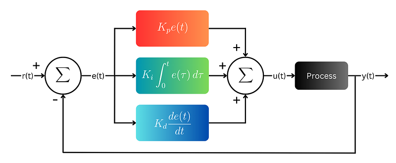
The control loop of a PID controller is presented in the block diagram above. r(t) is the setpoint and y(t) is the process variable. The process variable is subtracted from the setpoint to get the error signal, e(t).

The control signal, u(t), is the sum of the proportional, integral and derivative terms. The control signal is input to the process and this, in turn, causes the process variable to update.

The gradient descent algorithm

Gradient descent is an optimization algorithm commonly used in machine learning and mathematical optimization. It aims to find the minimum of a given cost function by iteratively adjusting the parameters based on the cost function gradient. The gradient points in the direction of the steepest ascent, so by taking steps in the opposite direction, the algorithm gradually converges towards the optimal solution.

A single gradient descent update step is defined as:

Where aₙ is a vector of input parameters. The subscript n denotes iteration. f(aₙ) is a multi-variable cost function and ∇f(a) is the gradient of that cost function. ∇f(aₙ) represents the direction of steepest ascent so it is subtracted from aₙ to reduce the cost function on the next iteration. 𝛾 is the learning rate which determines the step size at each iteration.

An appropriate value for 𝛾 must be selected. Too big and the steps taken at each iteration will be too large and cause the gradient descent algorithm to not converge. Too small and the gradient descent algorithm will be computationally expensive and take a long time to converge.

Gradient descent is applied in a wide range of fields and disciplines. In machine learning and deep learning, it is a fundamental optimization algorithm used to train neural networks and optimize their parameters. By iteratively updating the weights and biases of the network based on the gradient of the cost function, gradient descent enables the network to learn and improve its performance over time.

Beyond machine learning, gradient descent is utilized in various optimization problems across engineering, physics, economics, and other domains. It assists in parameter estimation, system identification, signal processing, image reconstruction, and many other tasks that require finding the minimum or maximum of a function. The versatility and effectiveness of gradient descent make it an essential tool for solving optimization problems and improving models and systems across diverse fields.

Optimizing PID controller gains using gradient descent

There are several methods available to tune a PID controller. These include the manual tuning method and heuristic methods like the Ziegler-Nichols method. The manual tuning method can be time-consuming and may require multiple iterations to find optimal values while the Ziegler-Nichols method often yields aggressive gains and large overshoot which means it is not suitable for certain applications.

Presented here is a gradient descent approach to PID controller optimization. We will optimize the control system of a car cruise control system subject to a step change in setpoint.

By controlling the pedal position, the controller’s objective is to accelerate the car up to the velocity setpoint with minimum overshoot, settling time and steady-state error.

The car is subject to a driving force proportional to the pedal position. Rolling resistance and aerodynamic drag forces act in the opposite direction to the driving force. Pedal position is controlled by the PID controller and limited to within a range of -50% to 100%. When the pedal position is negative, the car is braking.

It is helpful to have a model of the system when tuning PID controller gains. This is so that we can simulate the system response. For this I have implemented a Car class in Python:

import numpy as np

class Car:
    def __init__(self, mass, Crr, Cd, A, Fp):
        self.mass = mass # [kg]
        self.Crr = Crr # [-]
        self.Cd = Cd # [-]
        self.A = A # [m^2]
        self.Fp = Fp # [N/%]
    
    def get_acceleration(self, pedal, velocity):
        # Constants
        rho = 1.225 # [kg/m^3]
        g = 9.81 # [m/s^2]

        # Driving force
        driving_force = self.Fp * pedal

        # Rolling resistance force
        rolling_resistance_force = self.Crr * (self.mass * g)

        # Drag force
        drag_force = 0.5 * rho * (velocity ** 2) * self.Cd * self.A

        acceleration = (driving_force - rolling_resistance_force - drag_force) / self.mass
        return acceleration
    
    def simulate(self, nsteps, dt, velocity, setpoint, pid_controller):
        pedal_s = np.zeros(nsteps)
        velocity_s = np.zeros(nsteps)
        time = np.zeros(nsteps)
        velocity_s[0] = velocity

        for i in range(nsteps - 1):
            # Get pedal position [%]
            pedal = pid_controller.compute(setpoint, velocity, dt)
            pedal = np.clip(pedal, -50, 100)
            pedal_s[i] = pedal

            # Get acceleration
            acceleration = self.get_acceleration(pedal, velocity)
            
            # Get velocity
            velocity = velocity_s[i] + acceleration * dt
            velocity_s[i+1] = velocity

            time[i+1] = time[i] + dt
        
        return pedal_s, velocity_s, time

ThePIDController class is implemented as:

class PIDController:
    def __init__(self, Kp, Ki, Kd):
        self.Kp = Kp
        self.Ki = Ki
        self.Kd = Kd
        self.error_sum = 0
        self.last_error = 0
    
    def compute(self, setpoint, process_variable, dt):
        error = setpoint - process_variable
        
        # Proportional term
        P = self.Kp * error
        
        # Integral term
        self.error_sum += error * dt
        I = self.Ki * self.error_sum
        
        # Derivative term
        D = self.Kd * (error - self.last_error)
        self.last_error = error
        
        # PID output
        output = P + I + D
        
        return output

Taking this object-oriented programming approach makes it much easier to set up and run multiple simulations with different PID controller gains as we must do when running the gradient descent algorithm.

TheGradientDescent class is implemented as:

class GradientDescent:
    def __init__(self, a, learning_rate, cost_function, a_min=None, a_max=None):
        self.a = a
        self.learning_rate = learning_rate
        self.cost_function = cost_function
        self.a_min = a_min
        self.a_max = a_max
        self.G = np.zeros([len(a), len(a)])
        self.points = []
        self.result = []
    
    def grad(self, a):
        h = 0.0000001
        a_h = a + (np.eye(len(a)) * h)
        cost_function_at_a = self.cost_function(a)
        grad = []
        for i in range(0, len(a)):
            grad.append((self.cost_function(a_h[i]) - cost_function_at_a) / h)
        grad = np.array(grad)
        return grad
    
    def update_a(self, learning_rate, grad):
        if len(grad) == 1:
            grad = grad[0]
        self.a -= (learning_rate * grad)
        if (self.a_min is not None) or (self.a_max is not None):
            self.a = np.clip(self.a, self.a_min, self.a_max)
    
    def update_G(self, grad):
        self.G += np.outer(grad,grad.T)
    
    def execute(self, iterations):
        for i in range(0, iterations):
            self.points.append(list(self.a))
            self.result.append(self.cost_function(self.a))
            grad = self.grad(self.a)
            self.update_a(self.learning_rate, grad)
    
    def execute_adagrad(self, iterations):
        for i in range(0, iterations):
            self.points.append(list(self.a))
            self.result.append(self.cost_function(self.a))
            grad = self.grad(self.a)
            self.update_G(grad)
            learning_rate = self.learning_rate * np.diag(self.G)**(-0.5)
            self.update_a(learning_rate, grad)

The algorithm is run for a specified number of iterations by calling execute or execute_adagrad. The execute_adagrad method executes a modified form of gradient descent called AdaGrad (adaptive gradient descent).

AdaGrad has per-parameter learning rates that increase for sparse parameters and decrease for less sparse parameters. The learning rate is updated after each iteration based on a historical sum of the gradients squared.

We will use AdaGrad to optimize the PID controller gains for the car cruise control system. Using AdaGrad, the gradient descent update equation becomes:

Now we need to define our cost function. The cost function must take a vector of input parameters as input and return a single number; the cost. The objective of the car cruise control is to accelerate the car up to the velocity setpoint with minimum overshoot, settling time and steady-state error. There are many ways we could define the cost function based on this objective. Here we will define it as the integral of the error magnitude over time:

Since our cost function is an integral, we can visualize it as the area under the error magnitude curve. We expect to see the area under the curve reduce as we approach the global minimum. Programmatically, the cost function is defined as:

def car_cost_function(a):
    # Car parameters
    mass = 1000.0  # Mass of the car [kg]
    Cd = 0.2  # Drag coefficient []
    Crr = 0.02 # Rolling resistance []
    A = 2.5 # Frontal area of the car [m^2]
    Fp = 30 # Driving force per % pedal position [N/%]

    # PID controller parameters
    Kp = a[0]
    Ki = a[1]
    Kd = a[2]

    # Simulation parameters
    dt = 0.1  # Time step
    total_time = 60.0  # Total simulation time
    nsteps = int(total_time / dt)
    initial_velocity = 0.0  # Initial velocity of the car [m/s]
    target_velocity = 20.0 # Target velocity of the car [m/s]

    # Define Car and PIDController objects
    car = Car(mass, Crr, Cd, A, Fp)
    pid_controller = PIDController(Kp, Ki, Kd)

    # Run simulation
    pedal_s, velocity_s, time = car.simulate(nsteps, dt, initial_velocity, target_velocity, pid_controller)

    # Calculate cost
    cost = np.trapz(np.absolute(target_velocity - velocity_s), time)
    return cost

The cost function includes the simulation parameters. The simulation is run for 60 seconds. During this time we observe the response of the system to a step change in setpoint from 0 m/s to 20 m/s. By integrating error magnitude over time, the cost is calculated for every iteration.

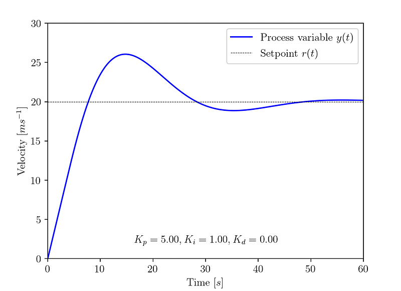
Now, all that is left to do is run the optimization. We will start with initial values of Kp = 5.0, Ki = 1.0 and Kd = 0.0. These values give a steady, oscillating response, with overshoot, that eventually converges to the setpoint. From this start point we will run the gradient descent algorithm for 500 iterations using a base learning rate of 𝛾=0.1:

a = np.array([5.0, 1.0, 0.0])
gradient_descent = GradientDescent(a, 0.1, car_cost_function, a_min=[0,0,0])
gradient_descent.execute_adagrad(500)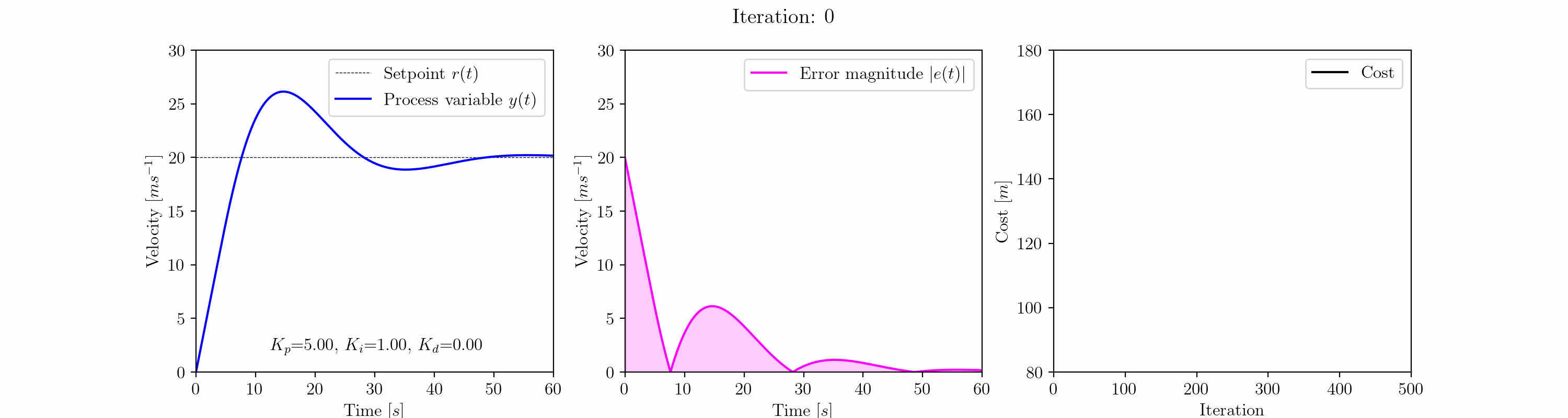

The animated plot above shows the evolution of the car cruise control step response as the gradient descent algorithm tunes the Kp, Ki and Kd gains of the PID controller.

By iteration 25, the gradient descent algorithm has eliminated the oscillatory response. After this point, something interesting happens. The algorithm wanders into a local minimum characterized by an overshoot of ~ 3 m/s. This happens in the region of 6.0 < Kp < 7.5, Ki ~= 0.5, Kd = 0.0 and lasts right up to iteration 300.

After iteration 300, the algorithm moves out of the local minimum to find a more satisfactory response closer to the global minimum. The response is now characterized by zero overshoot, fast settling time and near-zero steady-state error.

Running the gradient descent algorithm for 500 iterations we arrive at our optimized PID controller gains; Kp = 8.33, Ki = 0.12 and Kd = 0.00.

The proportional gain is still rising steadily. Running more iterations (not shown here), as Kp slowly increases, we find further reduction to the cost function is possible though this effect becomes increasingly marginal.

Summary

Adopting a method widely used for solving machine learning and deep learning problems, we have successfully optimized PID controller gains for a car cruise control system.

Starting with initial values of Kp = 5.0, Ki = 1.0 and Kd = 0.0 and applying the AdaGrad form of the gradient descent algorithm we observed how this low-dimension system first wanders into a local minimum before eventually finding a more satisfactory response with zero overshoot, fast settling time and near-zero steady-state error.

In this article, we have seen how gradient descent can be a powerful tool when applied to classic engineering optimization problems. Beyond the example presented here, gradient descent can be utilised to solve other engineering problems like inverse kinematics in robotics, topology optimization and many more.

Do you have an optimization problem that you think gradient descent could be applied to? Let me know in the comments below.

Enjoyed reading this article?

Follow and subscribe for more content like this — share it with your network — try applying gradient descent to your own optimization problems.

All images unless otherwise noted are by the author.

References

Web

[1] GitHub (2023), pid_controller_gradient_descent

[2] Wikipedia (2023), Ziegler–Nichols method (accessed 10th July 2023)