PERSONAL FINANCE

Personal Finance 101: An Easy Guide to Building A Budgeting and Expense Tracking Tool

Tracking expenses is the first step in financial literacy.

According to CareerBuilder, 78% of Americans live paycheck to paycheck.

This number may be exacerbated by the recent recession, which has resulted in millions of people not receiving their paycheck.

What can you do about it? How about you track your expenses and start a budget?

Tracking expenses is essential, it will help you gain awareness about your spending habits, and therefore, it will support you to optimize your spending. Expense tracking will answer the oldest question in finance — Where did the money go?

Budgeting allows you to allocate each dollar of your hard-earned money to a specific role. Budgeting empowers you to start an emergency fund, pay back debt, save for that downpayment, and many more.

There are many apps out there, which help in tracking expenses and budgeting. But, these apps cost money, are not tailored specifically for you, and can’t be updated easily if something changed in your financial situation.

Building your own budgeting and tracking tool is simple. It can be stored in a cloud service (google docs, dropbox, or iCloud) and accessed remotely from anywhere.

In the following, we will, step-by-step, build our very own budgeting and tracking tool in Excel. I chose Excel because:

• The formulas in excel are easy and do not require excessive knowledge in programming and coding.
• The formulas can easily be adapted for other software such as Numbers or Google Sheets.
• You can copy/paste cells to copy the formula for other cells.

NOTE THIS: The formulas I’ll be presenting in this post are for the English version of Excel. If you use Excel in a different language, please translate the equations to that language. Also, in my Excel version, I use ; as a separator in the formulas. Check which separator is used in your Excel version.

Before we start with building this tool, note down your recurring expenses — monthly, quarterly, semiannually, and annually. Also, note down your fixed monthly income — salary, income from real estate, etc.

To build the budgeting and expense tracking tool, we need to develop three sheets in excel:

1. The lists sheet — The name of this sheet has to be Lists.
2. the months’ sheets — January, February, …, December.
3. The overview sheet

The Lists Sheet

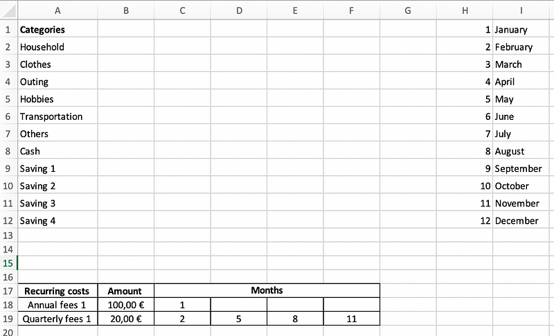
In this sheet, we will write down three lists required to program this tool. List 1: the categories for the monthly variable expenses, List 2: The months, List 3: the recurring charges. The lists are necessary for the further development of the tool.

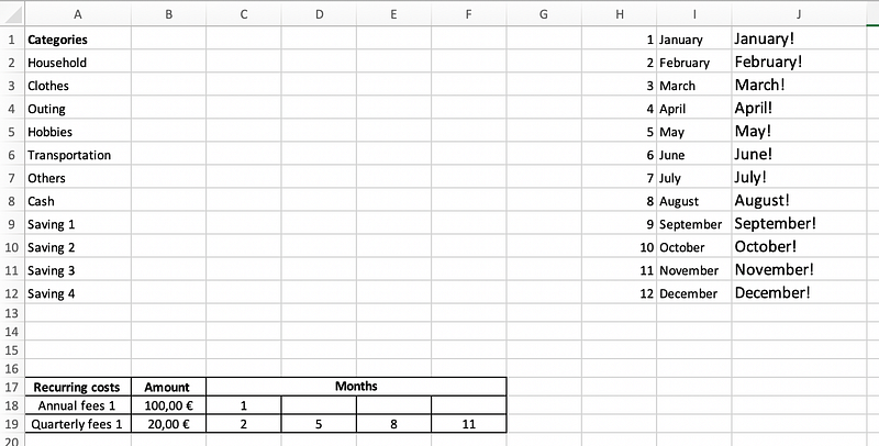
In cell J1 type the following formula =I1&"!”Then pull down from the right bottom corner of the cell. The result allows us to better reference in the upcoming steps.

The “Categories” list will be used as a dropdown menu later on. For this example, I’ve added four different savings categories (house, car, vacation, etc.). The “Cash” category tracks the withdrawn cash from the bank account. The list can be modified and extended as suitable.

The “Recurring costs” list includes charges, which are not monthly but can occur in quarterly, semiannually, or annually fashion. Write down the amounts and the months in which these charges arise, as shown in the screenshots.

The Months’ Sheets

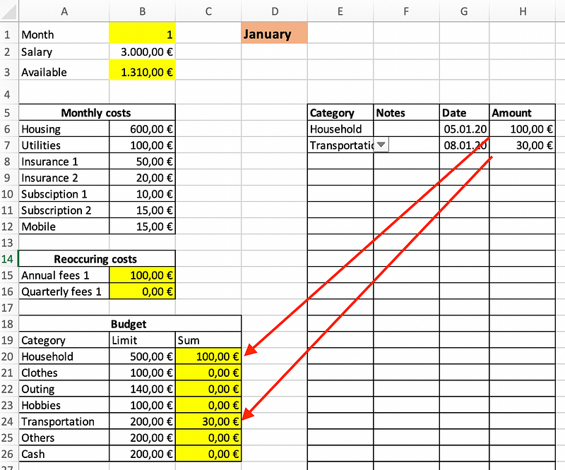
This sheet will be duplicated eleven times after we are done with the January sheet. Therefore, it is essential to make sure that the first sheet is current and includes everything. I filled the sheet as fits this example. The colored cells include equations and formulas.

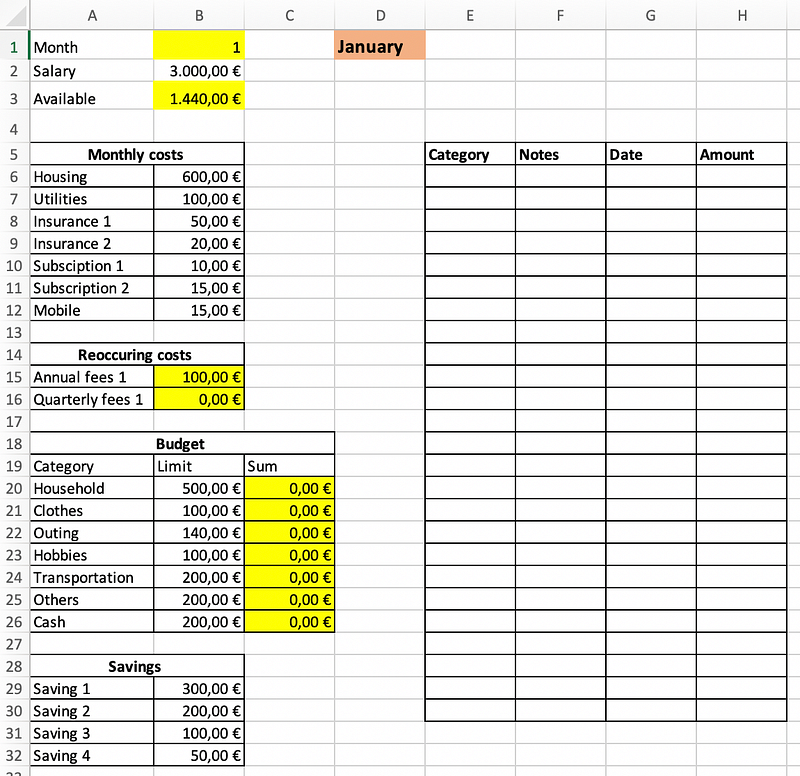
The formula in cell B3 is the simplest. Its goal is to calculate the available funds for the month. It subtracts all the costs and savings from the monthly salary.

=B2-SUM(B6:B12;B15:B16;C20:C26;B29:B32)

Cell B15 is a little bit tricky. The formula here outputs the recurring expenses based on the month. Annual fees 1 equals 100,00€ only in January. The formula checks the values of the month in cell B1 and compares the value with the months documented under the lists sheet.

=IF(OR($B$1=Lists!C18;$B$1=Lists!D18;$B$1=Lists!E18;$B$1=Lists!F18);Lists!B18;0)

This formula includes two functions: IF-function and OR-function. The OR function is true if only one of its variables is true. The If function gives a specific value if the function is true and another value if the function is false.

Cell B1 is referenced in this formula as $B$1 to prevent Excel from changing this reference if we copy/paste the cell B15 . Copy and Paste cell B15 to cell B16 and the equation shall look like

=IF(OR($B$1=Lists!C19;$B$1=Lists!D19;$B$1=Lists!E19;$B$1=Lists!F19);Lists!B19;0)

Notice how Excel changed all the other values to +1 but not the cell B1 .

Cell C20 gets an easy formula, which can be copied to all the cells from C20 to C26 . The used function is a SUMIF function, which only sums the values if a specific condition is true. The formula in cell C20 will sum all the variable expenses in the table on the right-hand side.

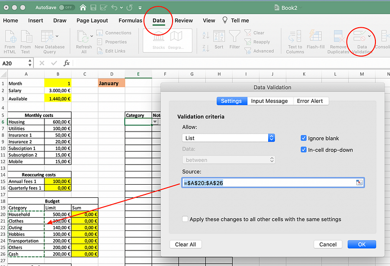
=SUMIF($E$6:$E$30;A20;$H$6:$H$30)

That is it, no more formulas or equations needed in the months’ sheets. Now, we only have to add a dropdown menu under the category column. to do this select cell E6 and select the Data tab, then Data validation, and then select the list as shown in the next figure.

That’s it! Easy isn’t it? There is one function that we can add, it is not a must, and it can function unproperly if saved on the cloud. The function is in cell D1 and cell B1 . This function saves one step of work. Instead of typing the month's number in cell B1 . With the help of this function, the value is written automatically based on the sheet's name.

In cell D1 type in

=MID(CELL(“filename”;A1);FIND(“]”;CELL(“filename”;A1))+1;256)

and in cell B1 type

=MONTH(DATEVALUE(D1&” 1"))

Now you only need to rename the sheet, and everything else is automated. Now every amount, which is written in the table on the right-hand side, is immediately considered in the budget and expense tracking tool.

These are the basics functions; you can add diagrams, conditional formatting, and even two different accounts if necessary. If you receive payments other than a fixed salary, you can add a category “Income.” Add the values in the table as negative values to consider them as income. Reformat the table and add as many functions as you wish, this is your budget and money tracking tool.

After you are done with January, just copy the sheet and rename it depending on the month.

The overview sheet

The overview sheet is not necessary. It functions only as a summary of all expenses and incomes in a given year. This is helpful if you are planning to use this tool for many years. I’ve been using this tool since 2016 now, with one Excel file per year saved to my Dropbox account.

A simple overview is as shown in the next figure. The green highlighted cells are essential. They contain the cell number from the months’ lists, which includes the required information.

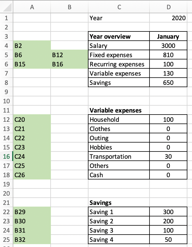
The required formulas for this sheet only reference a specific cell in the months’ sheets. The fixed charges and the recurring expenses are a sum.

The formula in Excel, which will get the salary information from all other sheets is

=@INDIRECT(VLOOKUP(D$3;Lists!$I$1:$J$12;2;FALSE)&$A4;TRUE)

Now copy/paste this cell to all other cells except for D5 to D8 . In D5 type in the following

=SUM(INDIRECT(VLOOKUP(D$3;Lists!$I$1:$J$12;2;FALSE)&$A5;TRUE):INDIRECT(VLOOKUP(D$3;Lists!$I$1:$J$12;2;FALSE)&$B5;TRUE))

Cell D5 can be copied to cell D6 , which now shall look like this

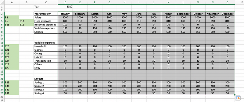
=SUM(INDIRECT(VLOOKUP(D$3;Lists!$I$1:$J$12;2;FALSE)&$A6;TRUE):INDIRECT(VLOOKUP(D$3;Lists!$I$1:$J$12;2;FALSE)&$B6;TRUE))

Cells D7 and D8 are just a Sum-function for the variable expenses and savings.

Select all the cells under January, including the month’s name, and drag it to the right for 11 further columns — Voilà! We are done.

Expense tracking and budgeting are the first steps in financial literacy. Each dollar has a task and cannot be relocated to another category.

Many apps and programs offer budgeting and Expense tracking services, however, these apps cost money (some cost even a monthly subscription fees) and are not tailored to your specific needs and situation.

Building your specific tool is simple and can be tailored to fit your requirements. You can update it later on with ease, and you don’t have to wait for a developer to release an update.

With my current Excel tool, I track my stocks, dividends, irregular income, home improvement costs, and all my investment portfolios across multiple platforms. No app can offer me this.

Walid Al Otaibi -WAO- works at an engineering company in Germany as a Project Manager. He manages mainly sustainable energy projects.

He comes from a multicultural background and is located in Germany since 2003. He is writing about Arab Culture, Multiculturalism, Finance, and Trending topics.