
Performance Comparison of SVM and ANN for Handwritten Character Recognition

Jinqi Ge
Harry Zheng
Abstract
Support Vector Machines(SVM) and Artificial Neural Networks(ANN) are among the most popular methods applied in various kind of pattern recognition. It is never an easy task for a machine to recognize letters, numbers, figures like humans being. Character recognition has become a challenging and fascinating topic in the field of image processing and machine learning. In this paper, we propose to recognize handwritten character by feedforward neural network and SVM classifier. Letter recognition dataset is used for training the SVM and ANN. Both methods are divided into training and testing phase. A comparative analysis and evaluation between two classifiers is presented with SVM and ANN. The experimental results suggest that comparing ANN, we reached a higher accuracy using SVM (RBF kernel) with an average rate of 94.2%.
Table of Contents
3.1 Support Vector Machines(SVM)
3.2 Artificial neural networks(ANN)
4 OVERVIEW OF SVM AND ANN RECOGNITION SYSTEM
4.1.3 Evaluating the performance of the model
4.1.4 Model performance tuning
4.2.1Installingnnetpackage&datasetclassification
1 Introduction
Recently, handwritten letter recognition has become one of the most challenging and popular research topic in the area of pattern recognition and artificial intelligence. This is due to the variety of handwritten styles, the lack of enough support information of source and the variations between different writers [1]. For these reasons, it is very hard to identified by a machine.
Several up-to-date methods and techniques were proposed to decrease the processing time and give more accurate recognition rate. In 2008, Malon and his team conducted a research on the Mathematical symbol recognition with SVM [2]. Support Vector Machine is adopted to classify several experimental mathematical symbols and improved the performance of InftReader method. The result was claimed that the SVM could bring the error rate down to 41%.
Another study comes from Rao and his team in 2016, who proposed a modified back propagation based method for optical character recognition [3]. This method dramatically reduced the error and reached 100% promising accuracy in Optical Character Recognition (OCR).
In the next study, research on letter recognition is proposed by Mahto, Bahtia and Sharma in 2015 [4]. To classify the handwritten letter of Gurmukhi, they introduced a new technique for combing the horizontal and vertical projection feature extraction. This empirical study use Support Vector Machine with linear and polynomial kernel and k-NN(k=1,3,5,7) to recognize the handwritten letters. The linear SVM classifier gives the best accuracy of 98.06% among different kernels.
Another researcher, Murthy and Hanmandlu developed a new method of zoning based feature extraction for hand-written letter recognition [5]. To achieve the best performance, they included the label of black pixel location. The result was claimed to give the accuracy of 98.5% accuracy with the proposed SVM method.
Based on those previous works, this paper aims to compare two most popular classifiers, an artificial neural network (ANN) without feature extraction and Support Vector Machine(SVM). The proposed ANN model in this paper is a standard feedforward neural network. For the SVM we proposed both linear and RBF kernel for comparion. Both Model consists of two parts, that is training and testing phase. The attributes in chosen datasets are used to train the model without feature extraction in the training phase. In the testing phase ANN and SVM classifier are used to recognize the letters.
Our experiments proposed to classify the English alphabet including 26 letters. For this purpose, our recognition system need the one-to-one correspondence number of outputs to represent the 26 letters. In ANN experiments we have analysed and compared different data approaches with various number of iterations and hidden neurons. The proposed recognition method gives better recognition accuracy after comparing the result.
In the rest of the paper, we first introduce the chosen dataset in section 2. Then in section 3, we present a brief description of the SVM and ANN classifier. In section 4, we present an overview of our experimental system design. Section 5 present the experimental results are comparative analysis. Conclusion and future works are given in the last section.
2 Dataset
The character data “Letter Recognition Data Set” was taken from the UCI Machine Learning Repository [6]. The samples character images were retrieved from 20 different fonts and each letter was randomly parsed with 20,000 unique records. Each record was transferred to 16 numerical attributes, which are ranges from 0 to 15 and represented by integers. Table 1 shows all the information of the letter and 16 attributes. We split the datasets of 20,000 records into two parts: the training dataset (16000 records, 80% of total dataset) and the testing (4000 records, 20% of total set).
3 Methodology
3.1 Support Vector Machines(SVM)
3.1.1 The cost function
The cost function (some place is called the loss function) is very important in every algorithm in machine learning. This is because the process of training model is the process of optimizing the cost function, the partial derivative of the cost function to each parameter is the gradient mentioned in the gradient descent, and the regularization term is added to the cost function when overfitting is prevented [7]. In the process of learning related algorithms, the understanding of the cost function is also deepening. Here is a brief summary.
1. What’s the cost function?
Suppose that the training sample(x,y), the model is h and the parameter is θ. h(θ) = θTx( θT is the transposing of θ).
1) In general, any function that can measure the difference between the values predicted by the model h(θ) and the true value y can be called the cost function C(θ). If there are many samples, the values of all the cost functions can be calculated and recorded as J (θ). Therefore, it is easy to get the following properties about the cost function [8].
- For each algorithm, the cost function is not unique.
- The cost function is a function of the parameter θ.
- The total cost function J (θ)can be used to evaluate the quality of the model. The cost function is smaller, which indicates the model and parameters are more consistent with the training sample(x, y).
- J (θ)is a scalar;
2) When we have identified the model h, everything we do behind is training the parameter θof model. So when does model training end? The cost function is also involved, and because the cost function is used to measure the model, our goal is, of course, to get the best model. Therefore, the process of training parameters is to change theta continuously, thus obtaining a smaller J (θ). Ideally, when we get the minimum value of the cost function J, we get the optimal parameter theta [8]:
For example, J (θ)= 0 indicates that our model perfectly matches the observed data without any error.
3) In the process of optimizing parameter theta, the most commonly used method is gradient descent. The gradient here is the partial derivative of the cost function J (θ) to θ1, θ2, …, θn. Because of the need for partial derivatives, we can get another property of the cost function:
When choosing a cost function, it is best to select functions that are differentiable to parameter theta (total differential exists, partial derivative must exist).
2. Common forms of cost functions
In logistic regression, the most commonly used function is the cross entropy (Cross Entropy), and cross entropy is a common cost function.
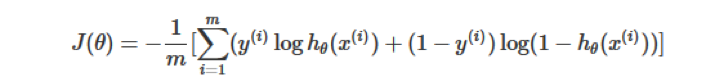
where
m: the number of training samples;
hθ(x): the yvalue predicted by parameter theta and X;
y: the yvalue of the original training sample, that is, the standard answer.
Upper corner sign (i): i-th sample.
The cost function measures the difference between the model predictive value h (θ)and the standard answer y, so the total cost function Jis the function of H (θ)and y, that is, J=f (h (θ), y). And because y is given in training samples, h (θ)is determined by θ, so eventually the change of model parameter theta leads to the change of J. Different theta, corresponding prediction value h (θ), also corresponds to the value of J of different cost functions. The process of change is:
θ→h(θ)→J(θ)
Theta causes the change of h (θ)and changes the value of J (θ).
3.1.2 Logistic regression
Before introducing logistic regression, we first briefly describe linear regression. The main idea of linear regression is to fit a straight line through historical data and use this line to predict the new data.
We know that the formula for linear regression is as follows [9]:

For logistic regression, the idea is also based on linear regression (Logistic Regression belongs to generalized linear regression model). The formula is as follows:
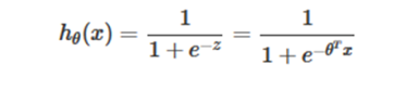
Especially,
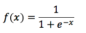
is known as the sigmoid function, we can see that the Logistic Regression algorithm maps the result of the linear function into the sigmoid function.
The Figure 1 of sigmoid function is as follow [10]:
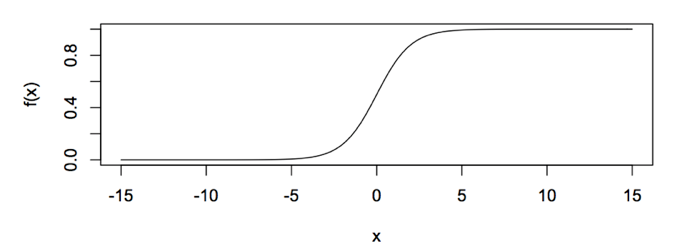
We can see that the output of sigmoid is between (0, 1) and the intermediate value is 0.5, so the meaning of the former formula h_θ (x) is well understood, because the h_θ (x) output is between (0, 1), and it also indicates the probability that the data belongs to a certain category, for example:
h_θ (x)<0.5 indicates that the current data is of Class A;
h_θ (x)>0.5 indicates that the current data is of Class B.
So we can regard the sigmoid function as the probability density function of sample data. With the above formula, what we need to do next is to estimate the parameter theta.
First of all, we see that the value of the θ function has a special meaning, which represents the probability that the h_θ (x) result takes 1, so the probability for the class 1 and Class 0 for the input xclassification results are [10]:
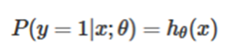
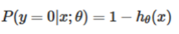
respectively.
Maximum likelihood estimation:
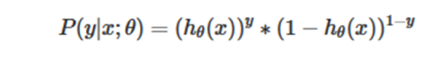
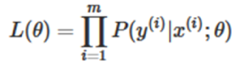
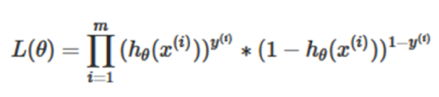
Based on the above formula, we can use the maximum likelihood estimation method in probability theory to solve the cost function. First, we get the probability function as follows [11]:
Because the sample data (m)are independent, their joint distribution can be expressed as the product of each marginal distribution, and the likelihood function is [11]:
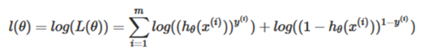
Taking logarithmic likelihood function [12]:
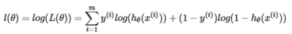
The maximum likelihood estimation is to get the value of θ that requires the maximum value of L(θ) to be obtained, which can be solved by the gradient ascent method. Let’s change it a little bit [12]:
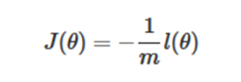
Since a negative coefficient 1/m is multiplied, the gradient descent algorithm can be used to solve the parameters.
1.1.1 Support vector machine
We wish to minimize SVM (support vector machine):
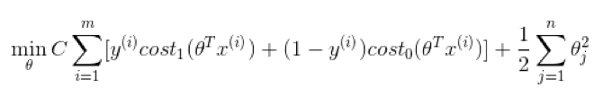
where
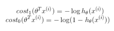
This is the definition of support vector machine in mathematics. It looks like the cost function J(θ), but adding a regularization term to the right. In a word, SVM is the problem of minimizing the above formula, thus obtaining the parameters C and θ.
Parameter θ is the form of hypothesis function of support vector machine.
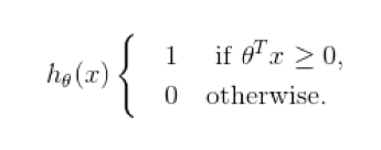
When you solve this optimization problem, and when you minimize the function of variables, you will get a very interesting decision boundary, SVM decision boundary:
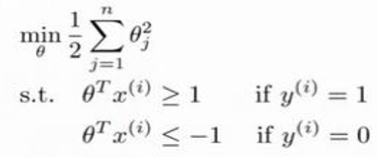
This is the boundary that classifies the samples.
3.2 Artificial neural networks(ANN)
An ANN is a model that can learn patterns from data by simulation the human nervous system [13]. They are applied in various scientific areas or solving engineering problems as to provide any non-linear function without being explicitly programmed.
The architecture of ANN used in this paper is the most popular feedforward artificial neural network. It has three layers: an input layer, one or several hidden layers and an output layer. The basic elements of each layer are named neurons. The letter recognition dataset has 16 attributes as input features and 26 capital letters (A to Z) as output labels, which represents 16 imputes and 26 outputs. Figure 2 is a typical simplified structure of ANN with 2 inputs, 3 hidden neurons and 1 output neuron.
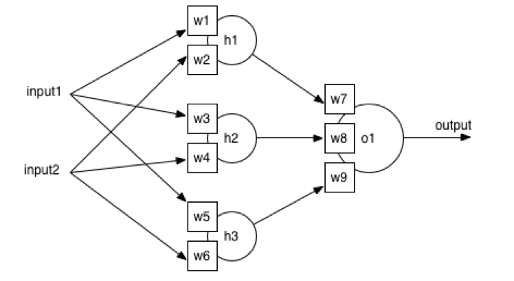
All above neurons have the same structure (Figure 3) and consist of two unit: a sum unit and a function unit. All of the weighted input value will be summarized and transfer to a single value x. Then the output of each neuron is called the output function or activation function. and represented with f(x).
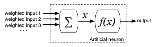
There are many output functions, including identity function or simple linear function. We use the most common one called sigmoid function which is already introduced before.
Then the output of each neuron can be calculated like the following formula based on the formal mentioned typical ANN structure [16]:
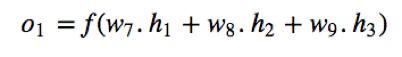
where:
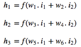
The example ANN is just doing a binary classification since it has only one output neuron. In our study that has 26 output neurons, each will be allocated to a class (capital letters from A to Z). Considering each output neuron allocated one sigmoid function, the output of our ANN is 26 numbers between 0 and 1. The class will then be recognized as the neuron which has the highest number.
To differentiate the output classes in ANN network, different weights are assigned to neuron inputs. Together with the input value, the weight of input neuron can hence determine the neuron’s output between 0 and 1 by the sigmoid function. The propose of the network training is to find the best value of weight to approach the most accurate classification.
The training algorithm is called backpropagation, which aims to updates all the weights with differences between the actual response and the function response. The training will be processed with a given number of iterations, until output a satisfied result with appropriate weights.
4 Overview of SVM and ANN recognition system
The proposed recognition system for the SVM and neural network was implemented using R 3.4.3.
4.1 SVM system
The flow of the proposed SVM recognition system is shown in Figure 4.
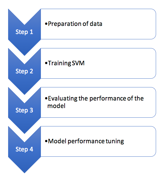
4.1.1 Preparation of data
Read the data into R, and confirm that the data received has 16 characteristics, which define the case of each letter class.
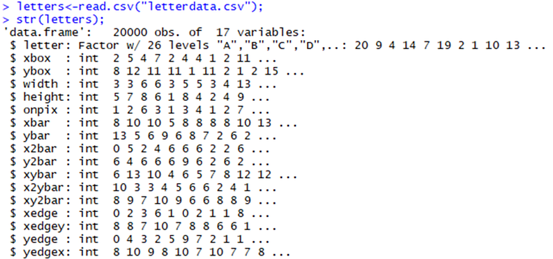
In this case, each feature is an integer. On the other hand, some of these integer variables appear to be quite wide, which seems to suggest the need for standardization or normalization of data, but fortunately, the R used to fit the support vector machine model will automatically help us to adjust the data.
Now we are entering the training and testing stage of machine learning process. I use the first 16000 records to build models and use the 4000 records to test them. We create training data frames and test data boxes. The code is as follows:

4.1.2 Training SVM
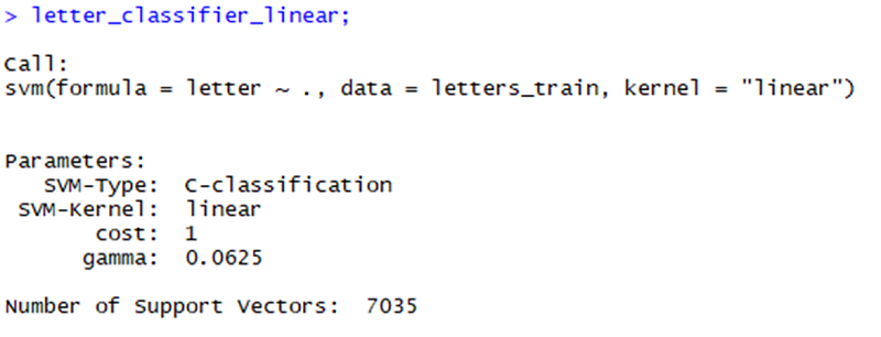
The e1071 package from the Statistics Department of Vienna University of Technology provides a R interface of the LIBSVM library, and then we call SVM () function based on training data. We start with training a simple linear support vector machine classifier and use the linear option to specify a linear kernel function.

Depending on computer performance, this operation may take some time to complete. When it is finished, input the name of the model to see some basic information about training parameters and the fitting degree of the model.
This information hardly tells us how well the model works in the real world. Therefore, we need to study the performance of the model based on the test data set, so as to determine whether it can be well extended to the unknown data.
4.1.3 Evaluating the performance of the model
The Predict () function allows us to predict based on the test data using the alphabetic classification model.

We need to compare the predicted values with the real values in the test data. For this purpose, we use the table () function. Only one part of the table is shown below.

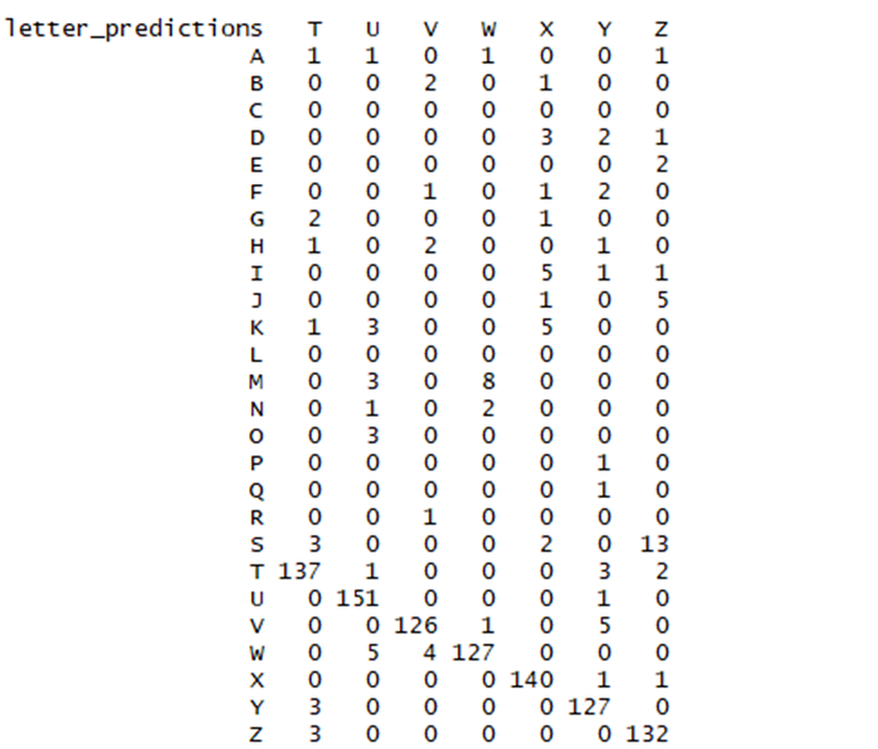
The diagonal value 137,151,126,127,140,127,132 represents the total number of records that match the predicted value with the true value. Similarly, the number of mistakes is also listed. For example, the value 3 in the Z row and the T column indicates that there are 3 cases where the letter T is mistaken for the letter Z.
A single look at each type of error may reveal some interesting patterns of specific letter types that are difficult for model identification, but it is also time consuming. Therefore, we can simplify our evaluation by calculating the accuracy of the whole, that is, only the letters that predict are correct or incorrect, and the types of errors are ignored.
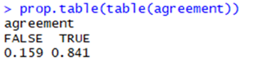
The following command returns a vector of TRUE or FALSE values to indicate whether the letter predicted by the model matches the real letter in the test data.

Using the table () function, we see that in the 4000 test records, there are 3364 letters correctly identified by the classifier.
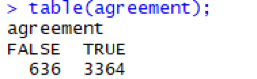
As a percentage, the accuracy is about 84.1%:
4.1.4 Model performance tuning
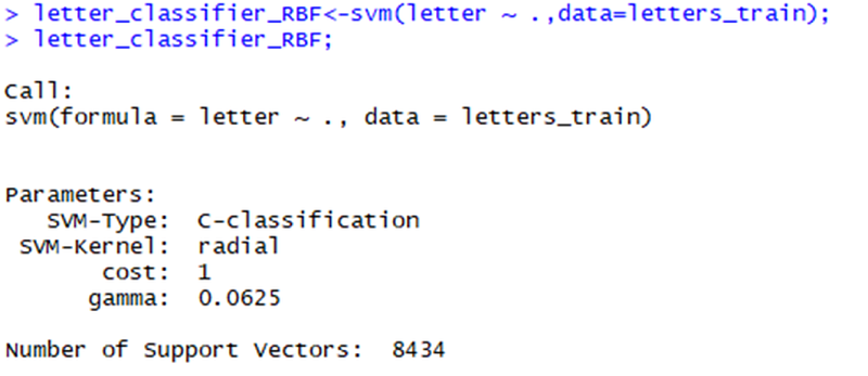
Previous support vector machines use simple linear kernel functions. By using a more complex kernel function, we can map data to a higher dimensional space, and it is possible to get a better degree of fitting. A popular practice is to start with the Gauss RBF kernel function, because it has proved to be able to run well for many types of data. We can use the SVM () function to train a RBF based support vector machine. The default kernel function of the SVM () function in e1071 is kernel = “radial” (RBF), so it does not need to be set, the code is shown as follows:
Then, we predict as before:

Finally, we compare the accuracy with our linear support vector machine.
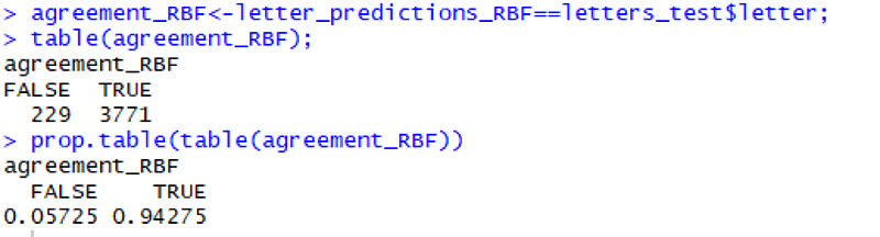
By changing the kernel function, we improved the accuracy of the character recognition model from 84.1% to 94.2%.
4.2 ANN system
Package nnet was adopted to realize feedforward artificial neural network, which has one hidden layer of sigmoid function neurons. Figure 5 shows the training and testing procedure of using nnet package in R.
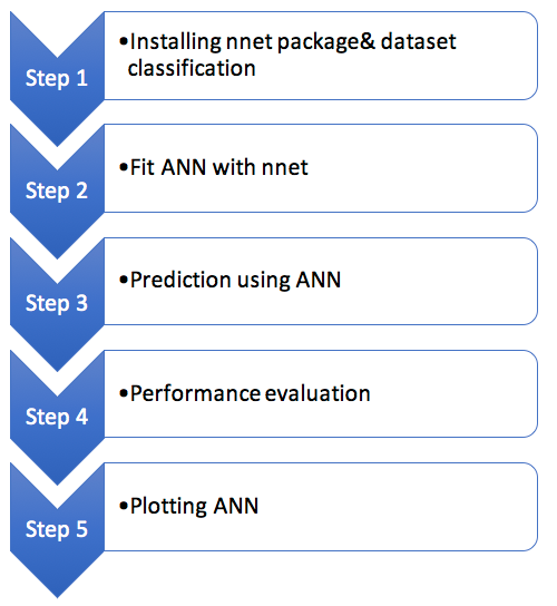
4.2.1 Installing nnet package & dataset classification
First the nnet should be installed and then load to RStudio. Then we need to load the source data and classified into trainset and testset with corresponding records descripted in section 2. The function is realized in R as follows:
install.packages(nnet)
library(nnet)
letters<- read.csv(“~/ML/letterdata.csv”)
trainset<-letters[1:16000, ];
testset<-letters[16001:20000, ];
4.2.2 Fit ANN with nnet
Although many parameters are fixed in nnet package, there are still some parameters for tuning to maximize the accuracy of classification. Table 2 shows the meanings and default values of the arguments used in our training procedure.
12 different neural networks architectures were chosen based on the mixed combination of parameters. Note that for ANN with large inputs, the parameter rang should set based on the following formula that:
In this experiment, we set rang based on the mentioned formula in 11 and 12 neural networks.
The training function is realized in R as follows:
letters.nn = nnet(letter ~ .,data = trainset,rang = 0.1,decay = 5e-4,size = 20,maxit = 5000)
4.2.3 Prediction using ANN
Then we use the trained ANN model to propose further prediction with testset. The result will be explained in detail in section 5. The predicting function is realized in R as follows:
## testset
letters.predict = predict(letters.nn,testset,type = “class”)
4.2.4 Performance evaluation
In this part, we need to evaluate the performance of the network module. Also the comparative analysis will present in section 6. In R system this is realized using the function confusionMatrix as follows:
# use union to ensure similar levels
u = union(testset$letter,letters.predict)
nn.table = table(factor(letters.predict, u), factor(testset$letter, u))
# Evaluate the result
confusionMatrix(nn.table)
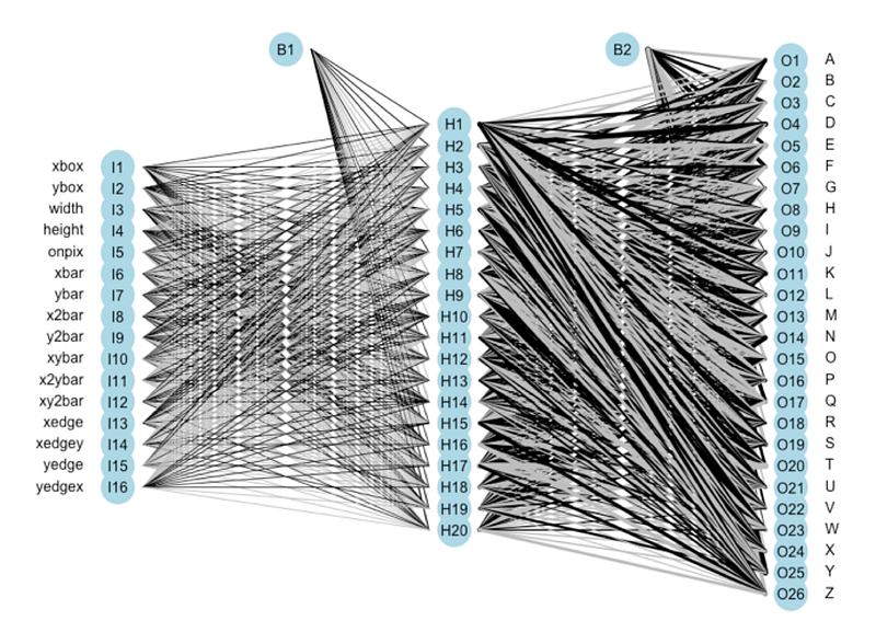
4.2.5 Plotting ANN
Figure 6 shows one of the ANN structureadopted in our test with 20 neurons in hidden layer. Note the bias neurons B1 and B2 added in hidden layer and output layer to allow the neural network to change the output value on demand. Also, larger weights will be showed with thicker lines and color indicates sign, that is black and grey represents positive and negative prediction value respectively [18].
This is realized with the function plotnet in R as follows:
#plot nn
library(NeuralNetTools)
plotnet(letters.nn)
5 Results & Discussion
5.1 SVM system evaluation
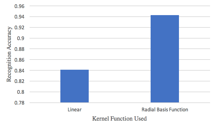
The following table shows the prediction results of single character recognition of 2 SVM classifiers. The statistics data showed the recognition accuracy of each classification of A~Z letters. We can conclude that 23/26 of recognition accuracy of SVM with radial basis function kernel are over 90%, which obviously presents the better performance than linear SVM.
Table 5 present the recognition result of two SVM system with linear and radial basis function(RBF) kernel, where the SVM classifier with radial basis function(RBF) kernel shows better accuracy.
Figure 7 shows the recognition accuracy result of above two SVM approaches. The SVM with rbf kernel performs obviously better than the linear SVM, more than ten percentage.
5.2 ANN system evaluation
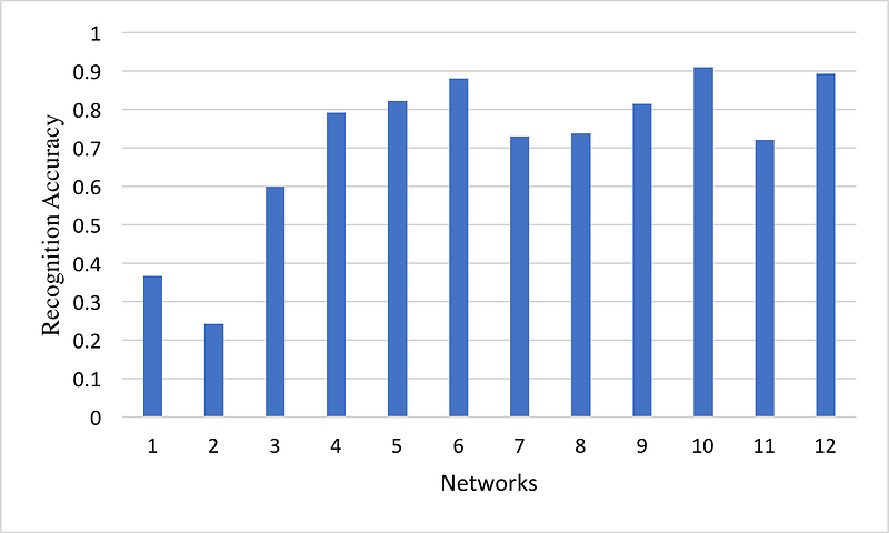
Table 6 shows the prediction result of the 12 ANN. The statistics data showed the recognition accuracy of each classification of A~Z letters and total result. We can conclude that the networks 10 presents the best performance.
Figure 8 shows the recognition accuracy total result of all 12 ANN approaches. However, only one of them obtains over 90% accuracy of recognition.
5.3 Compare ANN& SVM
The result in Table 7 shows that SVM with Kernel function of Radial Basis Function(RBF) performs better than Artificial Neural Network.
Figure 9 also visualized the comparing result.
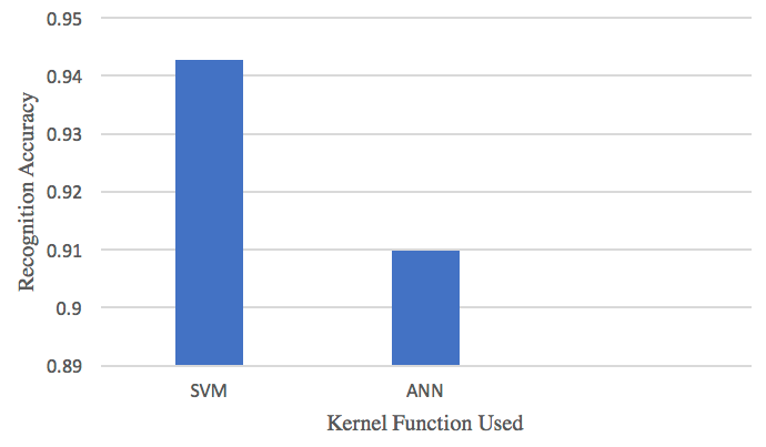
In our report, we use 2 support vector machines and 12 neural network classifiers. When we use a linear kernel function support vector machine classifier, it can correctly identify the alphabet accuracy of 84.1%, which is better than the 9 neural network classifier; while we use the RBF kernel function support vector. The accuracy of the classifier is 94.2%, which exceeds all 12 neural network classifiers. This result shows that SVM should be an advantage for small samples, and it is indeed one of the best classifiers.
Support vector machine is based on statistical theory, so it has strict theoretical and mathematical basis, not like neural network structure design need to rely on the designer’s experience knowledge and prior knowledge. Compared with neural network learning methods, Support vector machine has advantages:
1) Support vector machine (SVM) is based on SRM (structural risk minimization) principle, having good generalization ability.
2) By mapping the nonlinear problem in the input space to the high-dimensional space by constructing the kernel function, the linear function is constructed in the high-dimensional space.
3) The algorithm can be transformed into a convex optimization problem, which guarantees the global optimality of the algorithm and avoids the local minimum problem which the neural network can not solve.
4) Support vector machine has strict theoretical and mathematical foundation, avoiding the empirical components in neural network implementation.
6 Conclusion
Support vector machine (SVM) is a new generation learning machine based on statistical learning theory. It has many attractive features. It is superior to the traditional artificial neural network in function expression, popularization and learning efficiency.
Since SVM is used to solve support vectors with the aid of the quadratic programming, which will involve the calculation of the m order matrix (m is the number of samples). When the number of m is large, the storage and calculation of the matrix will consume a large amount of machine memory and operation time.
The main improvements to the above problems include J.Platt’s SMO algorithm, T.Joachims’ PCGC, Zhang ‘s CSVM, and O.L.Mangasarian’s SOR.
In the report, we have studied two machine learning methods that can provide great potential in letters recognition and classification. Result shows that comparing with Artificial neural networks(ANN),Support vector machine (SVM) has better approximation ability and generalization ability. Future research on the application of Support vector machine (SVM) will spur greater interest in various fields for its unique superiority.
7 Bibliography
[1]M. R. Phangtriastu, Jeklin Harefa and Dian Felita Tanoto, “Comparison Between Neural Network and Support Vector Machine in Optical Character Recognition,” Procedia Computer Science, vol. 116, pp. 351–357, 2017.
[2]Malon C, Uchida S and Suzuki M, “Mathematical symbol recognition with support vector machines,” 2008. [Online]. Available: http://www.sciencedirect.com/science/article/pii/S0167865508000603.
[3]Rao NV and Pradesh A, “OPTICAL CHARACTER RECOGNITION TECHNIQUE,” Technology AI, vol. 83, no. 2, 2016.
[4]Mahto MK, Bhatia K and Sharma RK, “Combined horizontal and vertical projection feature extraction technique for Gurmukhi handwritten character recognition,” in 2015 International Conference on Advances in Computer Engineering and Applications, 2015.
[5]M. OVR, “Zoning based Devanagari Character Recognition,” vol. 27, no. 4, p. 21–5, 2011.
[6]C. L. Blake and C. J. Merz, “UCI repository of machine learning databases,” 1998. [Online]. Available: https://archive.ics.uci.edu/ml/datasets/letter+recognition.
[7]J. Bell, “Support vector machines,” Machine Learning: Hands-On for Developers and Technical Professionals, pp. 139–160, 2014.
[8]Nasrabadi and N. M, “Pattern recognition and machine learning,” Journal of electronic imaging , vol. 049901, no. 16, p. 4, 2007.
[9]R. E. Schapire, “The boosting approach to machine learning: An overview,” Nonlinear estimation and classification, pp. 149–171, 2003.
[10]Dreiseitl, Stephan and Lucila Ohno-Machado, “Logistic regression and artificial neural network classification models: a methodology review,” Journal of biomedical informatics, vol. 35, no. 5–6, pp. 352–359, 2002.
[11]C. Robert, “Machine learning, a probabilistic perspective,” pp. 62–63, 2014.
[12]Jordan, Michael I. and Tom M. Mitchell, “Machine learning: Trends, perspectives, and prospects,” Science, vol. 349, no. 6245 , pp. 255–260, 2015.
[13]Gazzah, Sami and Najoua Ben Amara, “Neural networks and support vector machines classifiers for writer identification using Arabic script,” International Arab Journal of Information Technology (IAJIT), vol. 5, p. 1, 2008.
[14]V. D. Do and Dong-Min Woo, “Handwritten Character Recognition Using Feedforward Artificial Neural Network,” in 7th International Conference on Latest Trends in Engineering & Technology, Pretoria, 2015.
[15]Kumar, Parveen, N. Sharma and A. Rana, “Handwritten Character Recognition using Different Kernel based SVM Classifier and MLP Neural Network (A COMPARISON),” International Journal of Computer Applications, vol. 53, no. 11, 2012.
[16]S. D. B. M. N. L. M. M. K. a. D. K. B. Arora, “Performance comparison of SVM and ANN for handwritten Devnagari character recognition,” vol. 1006, no. 5902, 2010.
[17]Brian Ripley and William Venables, “Feed-Forward Neural Networks and Multinomial Log-Linear Models,” 2 2 2016. [Online]. Available: https://cran.r-project.org/web/packages/nnet/nnet.pdf. [Accessed 4 6 2018].
[18]S. Thompson, “Visualizing neural networks in R — update,” 4 3 2013. [Online]. Available: https://beckmw.wordpress.com/tag/nnet/. [Accessed 4 6 2018].