Parquet Best Practices: The Art of Filtering

Understanding how to filter Parquet files

If you like to experience Medium yourself, consider supporting me and thousands of other writers by signing up for a membership. It only costs $5 per month, it supports us, writers, greatly, and you get to access all the amazing stories on Medium.

This article assumes you have basic knowledge of Parquet files. If not, you can check my other articles on Parquet, such as Introduction to Parquet and Parquet Metadata.

If you want to reproduce the input data for this article, the code can be found at the end.

Filtering in Parquet involves selecting specific rows from a Parquet file based on a certain condition. This reduces the amount of data that needs to be read and processed, leading to significant improvements in the performance of big data applications.

One of the main benefits of Apache Parquet is its ability to store data in a columnar format. Each column is stored separately and can be read independently, enabling efficient filtering through column pruning. Only the columns required for the filter condition are read.

Additionally, performance can be improved through the use of two techniques: partition pruning and predicate pushdown. Partition pruning operates on the partitions, while predicate pushdown allows for filtering the data before it is read using Metadata.

In this article, we will discuss the concepts behind Parquet filtering as well as provide examples of how to profit from column pruning, partition pruning, and predicate pushdown in order to filter Parquet files efficiently.

Whether you are a Data Scientist, Data Engineer, or Data Analyst, this article will provide you with the knowledge and tools you need to filter large datasets using Parquet efficiently.

Parquet filtering with examples

When we filter Parquet files, we rely on one explicit method, which is column pruning, and two underlying concepts that are crucial to understanding what is happening underhood partition pruning and predicate pushdown.

To explore those concepts, we provide you with a case study in which a Data Engineer has provided you with loan applicants’ data, and you need to load the data efficiently because it is huge Data.

The import packages you will need:

import pyarrow as pa
import pyarrow.parquet as pq
import pandas as pd
import numpy as np
import time
import os

Columns pruning

Column pruning is a method of reducing the amount of data that needs to be read and processed during filtering by only reading the columns that are required for the filter condition. This is possible due to the columnar storage format of Parquet, which allows individual columns to be read independently of one another.

In order to apply column pruning, it is important to know the available columns in the data. To do this, the schema of the first Parquet file in the folder APPLICATIONS_PARTITIONED can be read. This will provide the necessary information to only read the required columns during the filtering process, which will improve performance by reducing the amount of data that needs to be processed.

def get_first_parquet_from_path(path):
    for (dir_path, _, files) in os.walk(path):
        for f in files:
            if f.endswith(".parquet"):
                first_pq_path = os.path.join(dir_path, f)
                return first_pq_path
path = 'APPLICATIONS_PARTITIONED'
first_pq = get_first_parquet_from_path(path)
pq.read_schema(first_pq)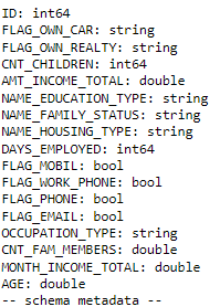

Let’s apply column pruning to our dataset and filter for only variables of interest: ‘ID’, ‘CNT_CHILDREN’, ‘DAYS_EMPLOYED’, and ‘AMT_INCOME_TOTAL’. It is very simple, we just need to fill the columns argument:

cols=['ID', 'CNT_CHILDREN', 'DAYS_EMPLOYED', 'AMT_INCOME_TOTAL']
df=pd.read_parquet('APPLICATIONS_PARTITIONED', columns=cols)
df.head()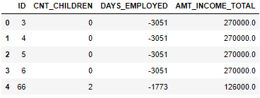

As we see the DataFrame loaded just contains our variables of interest.

Let’s also compare the run-time of partition pruning with the run-time of reading all the Parquet and filtering after.

cols=['ID', 'CNT_CHILDREN', 'DAYS_EMPLOYED', 'AMT_INCOME_TOTAL']
start_time = time.time()
df=pd.read_parquet('APPLICATIONS_PARTITIONED', columns=cols)
print(f'{np.round(time.time() - start_time, 2)} seconds with column pruning')

start_time = time.time()
df_slow = pd.read_parquet('APPLICATIONS_PARTITIONED')[cols]
print(f'{np.round(time.time() - start_time, 2)} seconds for the slow version of loading all and filtering after')

It is more than 10 times faster by loading only the columns that we are interested in, taking advantage of the column pruning instead of loading all the data and filtering it afterward.

Partition pruning

Partition pruning is a technique to enhance the efficiency of queries on partitioned data by skipping over partitions that are not relevant to the query. In Parquet, the data is organized into partitions based on one or more columns, known as partition keys or partition columns, using a directory structure.

When executing a query, the query optimizer analyzes the filter conditions and identifies the partitions that are relevant to the query. By skipping over non-relevant partitions, the amount of data that needs to be read and processed is reduced, thus significantly improving query performance, especially for large datasets.

In our dataset, we can find out the partitions by using my custom function to discover all the partitions in a directory:

def get_all_partitions(path):
    partitions = {}
    i = 0
    for (_, partitions_layer, _) in os.walk(path):
        if len(partitions_layer)>0:
            key = partitions_layer[0].split('=')[0]
            partitions[key] = sorted([partitions_layer[i].split('=')[1] for i in range(len(partitions_layer))])
        else:
            break
    return partitions
ps = get_all_partitions('APPLICATIONS_PARTITIONED')
ps.keys(), ps.values()

Based on the key results of the function, they are 2 layers of partitions, NAME_INCOME_TYPE and CODE_GENDER, and we have the values to filter them.

Since we are only interested in let’s say ‘Pensioner’ and ‘Working’ from NAME_INCOME_TYPE let’s only read these partitions.

cols = ['ID', 'CNT_CHILDREN', 'DAYS_EMPLOYED', 'AMT_INCOME_TOTAL']
filter_part = [('NAME_INCOME_TYPE', 'in', ('Pensioner', 'Working'))]
start_time = time.time()
df_pp = pd.read_parquet('APPLICATIONS_PARTITIONED', columns=cols, filters=filter_part)
print(f'{np.round(time.time() - start_time, 2)} seconds with columns pruning and partition pruning')

start_time = time.time()
df_pp_slow = pd.read_parquet('APPLICATIONS_PARTITIONED', columns=cols+['NAME_INCOME_TYPE'])
df_pp_slow = df_pp_slow[df_pp_slow['NAME_INCOME_TYPE'].isin(['Pensioner', 'Working'])]
print(f'{np.round(time.time() - start_time, 2)} seconds with columns pruning + filtering afterwards')

By providing the filters argument in order to profit also from partition pruning, we reduced our time from 0.91 to 0.51 seconds. And compared to columns pruning + filtering afterward, we still have a run-time reduced by nearly 4.

When using the filters argument, you have to provide a list of tuples, where the second element of each tuple is an operator.

I give you the list of all possible operators:

= or ==, !=, <, >, <=, >=, in and not in.

Those operators are great but you may ask yourself how to also do a filter involving the OR operator.

The solution is to include multiples lists in the list, which will be interpreted as having an OR condition.

Here’s an example where I filter on NAME_INCOME_TYPE = ‘Pensioner’ OR CODE_GENDER=’F’:

filter_part = [[('NAME_INCOME_TYPE', 'in', ('Pensioner', 'working'))],[('CODE_GENDER','=','F')]]
df_pp2 = pd.read_parquet('APPLICATIONS_PARTITIONED', columns=cols, filters=filter_part)

You have now learned how to take advantage of column pruning and partition pruning, but there is one last type of filtering you may want to do. Suppose you want to filter on a value within the dataset rather than the partitions. How to do that?

Predicate pushdown

Predicate pushdown is a technique used to filter data at the storage layer before it is read into memory. This is achieved by pushing the filtering conditions from the query down to the storage layer so that the storage layer can filter the data using the statistics found in the Metadata, reducing the amount of data that needs to be read and processed and improving query performance.

The utilization of predicate pushdown is similar to that of partition pruning with column filtering. A large part of the work is performed under the hood by Apache Parquet, which checks the filter argument list and constructs two internal lists:

• one for filters related to partitions for applying partition pruning
• one for filters related to in-file filtering where predicate pushdown will be applied.

Let me show you an example where predicate pushdown is in action. Suppose we want to find households that earn more than 250k a year. We will construct the filter using a condition on the variable AMT_INCOME_TOTAL, just as before.

cols = ['ID', 'CNT_CHILDREN', 'DAYS_EMPLOYED', 'AMT_INCOME_TOTAL']
filter_part = [('AMT_INCOME_TOTAL','>', 250000)]
start_time = time.time()
df_pp3 = pd.read_parquet('APPLICATIONS_PARTITIONED', columns=cols, filters=filter_part)
print(f'{np.round(time.time() - start_time, 2)} seconds with Column pruning and Predicate Pushdown')

I set the threshold at 250k to obtain roughly the same number of rows as when I read the data using column pruning and partition pruning:

print(df_pp.shape)
print(df_pp3.shape)

It is nearly the same size meaning that the difference in speed between partition pruning and predicate pushdown should only be due to the fact that predicate pushdown is more costly because it has to loop on every partition and then get the filtered data on each Parquet file, which is most costly than just reading a specified partition.

However, as you see 1.02 seconds is still fast because the files are smartly read thanks to the Metadata available in each file.

Still, we need to compare it to the case where we reproduce the same output without profiting from predicate pushdown:

It’s nearly the same size, so the difference in speed between partition pruning and predicate pushdown is only due to the fact that predicate pushdown is more expensive. This is because it has to iterate through each partition and then retrieve the filtered data from each Parquet file, which is more costly than simply reading a specified partition.

However, 1.02 seconds is still a fast time, as the files are read efficiently due to the metadata available in each file.

We still need to compare this to the case where we produce the same output without benefiting from predicate pushdown.

cols = ['ID', 'CNT_CHILDREN', 'DAYS_EMPLOYED', 'AMT_INCOME_TOTAL']
filter_part = [('AMT_INCOME_TOTAL','>', 250000)]
start_time = time.time()
df_slow = pd.read_parquet('APPLICATIONS_PARTITIONED', columns=cols)
df_slow = df_slow.loc[(df_slow['AMT_INCOME_TOTAL']>250000), cols]
print(f'{np.round(time.time() - start_time, 2)} seconds without profiting from predicate pushdown')

As we expected, the gain in run-time is not as important as the columns pruning or partition pruning, but we still get a run-time lower by profiting from predicate pushdown.

Conclusion

In this article, we explored the concepts behind filtering in Parquet files. Specifically, we covered column pruning, partition pruning, and predicate pushdown. By gaining a deeper understanding of these techniques, you are now equipped to efficiently filter large Parquet files. Through practical examples, we applied these concepts and showed how to effectively take advantage of them to filter data.

The full code to generate the input data we used:

## Bash command
pip install kaggle
kaggle datasets download -d rikdifos/credit-card-approval-prediction
shutil.unpack_archive('credit-card-approval-prediction.zip')

## Python code
applications = pd.read_csv('application_record.csv')
applications = pd.concat(10*[applications]).reset_index().drop(columns=['ID','index']).reset_index().rename(columns={'index':'ID'})
applications['MONTH_INCOME_TOTAL'] = applications['AMT_INCOME_TOTAL']/12
applications['AGE'] = - np.floor(applications['DAYS_BIRTH']/365)
my_schema = pa.Schema.from_pandas(applications)
my_schema = my_schema.set(12, pa.field('FLAG_MOBIL', 'bool'))
my_schema = my_schema.set(13, pa.field('FLAG_WORK_PHONE', 'bool'))
my_schema = my_schema.set(14, pa.field('FLAG_PHONE', 'bool'))
my_schema = my_schema.set(15, pa.field('FLAG_EMAIL', 'bool'))
my_schema = my_schema.remove(10)
applications.to_parquet('APPLICATIONS_PARTITIONED', schema = my_schema, partition_cols=['NAME_INCOME_TYPE', 'CODE_GENDER'])

Continue your learning with my other Parquet articles:

With no extra costs, you can subscribe to Medium via my referral link.

Or you can get all my posts in your inbox. Do that here!