
Pareto Distributions and Monte Carlo Simulations
Modelling web page views with a Pareto Distribution
Pareto Distributions are all around us. It has also been referred to as the 80/20 rule. As some examples:
- 20% of all websites get 80% of the traffic.
- The top 20% of earners globally make 80% of the income.
- You wear 20% of your clothes 80% of the time.
Traditionally, we are thought that the assumed distribution for a statistical range is a normal distribution, i.e. one where the mean = median = mode.
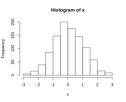
However, many of the phenomena we observe around us often more closely resemble a Pareto distribution.
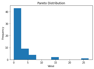
In this particular example, we can see a distribution that is heavily right-tailed, i.e. most of the observations with lower values (as defined by the x-axis) tend to the left of the graph, while a select few observations with higher values tend towards the right of the graph.
Modelling Web Page Views with a Monte Carlo Simulation
Let’s take the example of web page views over time. Here is a line graph showing fluctuations over time for the term “earthquake” from January 2016 — August 2020 from Wikimedia Toolforge:
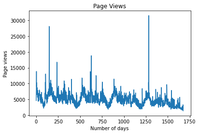
We can see that there are “spikes” in page views at certain periods — possibly at a time when an earthquake is under way somewhere in the world.
This is what we would expect — this is an example of a search term which sees higher page view interest at certain times. As a matter of fact, many webpages follow this pattern, where traffic more or less follows a stationary pattern — accompanied by sudden “spikes”.
Let’s plot a histogram of this data.
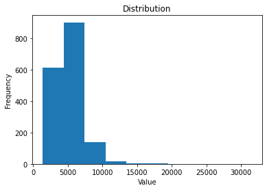
In the above instance, we see that the majority of page views for a given day are below 10,000, while there are a select few incidences where this is exceeded.
The maximum number of page views in a given day over the selected time period was 31,520. This closely represents a Pareto Distribution.
Attempting to forecast page views with traditional time series tools such as ARIMA is quite futile. This is because it is not possible to know in advance when a particular spike in traffic will occur — as it is heavily dependent on external circumstances and not related to past data.
A more meaningful exercise would be to run simulations to forecast the range of traffic that one might expect to see given the assumption of a Pareto distribution.
The Pareto Distribution is called in Python as follows:
numpy.random.pareto(a, size=None)a represents the shape of the distribution, and size is set to 10,000, i.e. 10,000 random numbers from the distribution are generated for the Monte Carlo simulation.
The mean and standard deviation for the original time series are calculated.
mu=np.mean(value)
sigma=np.std(value)
The time series has a mean of 5224 and a standard deviation of 2057.
Using these values, a Monte Carlo simulation can be generated using these parameters, along with the random sampling from an assumed Pareto distribution.
t = np.random.pareto(a, 10000) * (mu+sigma)
t
As mentioned, the value of a is dependent on the shape of the distribution. Let’s set this to 3 in the first instance.
Here are the recorded values for the distribution in percentile terms:
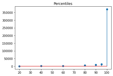
We can see that the maximum value recorded when a = 3 is in excess of 350,000, which is far higher than the maximum recorded by the time series.
What happens if we set a = 4?
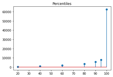
We now see that the maximum recorded value is now in excess of 60,000, which is still a lot higher than the maximum recorded by the time series.
Let’s try a = 5.
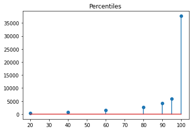
Interpretation
Maximum page views are just above 35,000, which is more in line with what we have seen in the original time series.
However, consider that in this case — we are only looking at time series data from 2016 onwards. Many of the most serious earthquakes actually happened before 2016.
For instance, let us suppose that an earthquake as serious as that of the 2004 Indian Ocean earthquake and tsunami were to happen today — we would reasonably expect that page view interest for the term “earthquake” would be much larger than that which we have observed since 2016.
If we assume that the Pareto distribution has a = 3, then the model is indicating that page views for this term could spike to in excess of 350,000.
In this regard, the Monte Carlo simulation is allowing us to examine scenarios that would be beyond the bounds of the time series data that has been recorded.
Earthquakes (unfortunately) have been around for a lot longer than the internet has — and therefore we have no way of measuring what page views for this search term would have been like during times where the most powerful earthquakes were recorded.
That said, conducting a Monte Carlo Simulation in conjunction with modelling on the closest theoretical distribution can allow for a strong scenario analysis of what the bounds of a time series could be under particular circumstances.
Conclusion
In this article, you have seen:
- What is a Pareto Distribution
- How to generate such a distribution in Python
- How to combine a Pareto distribution with a Monte Carlo simulation
Many thanks for your time. As always, very grateful for any feedback, thoughts, or indeed questions. Please feel free to leave them in the comments section.
Disclaimer: This article is written on an “as is” basis and without warranty. It was written with the intention of providing an overview of data science concepts, and should not be interpreted as professional advice in any way.