Pandas Crash Course: Top 30 Functions for Any Data Analysis

Become a Pro in using Pandas for Data Science

Embarking on a data analysis journey often leads us to Pandas, the powerhouse library that transforms the way we handle and manipulate data in Python.

In this crash course, we’ll unravel the top 30 Pandas functions that serve as the backbone for any data analysis task. Whether you’re a seasoned data scientist or a beginner navigating the world of data, these functions will become your go-to functions for any data analysis.

To illustrate the use of the top 30 Pandas functions, we’ll create a simple DataFrame using a hypothetical real-world dataset. In this example, let’s consider a dataset related to sales transactions.

import pandas as pd
import numpy as np

# Creating a hypothetical sales dataset
data = {
    'Date': pd.date_range(start='2023-01-01', end='2023-01-10'),
    'Product': ['A', 'B', 'A', 'C', 'B', 'A', 'C', 'A', 'B', 'C'],
    'Sales': [100, 150, 120, 80, 200, 110, 90, 130, 160, 75],
    'Region': ['North', 'South', 'East', 'West', 'North', 'South', 'West', 'North', 'East', 'South']
}
df = pd.DataFrame(data)
print("Original DataFrame:")
print(df)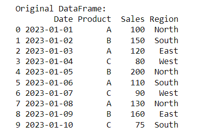

Now, let’s apply the Pandas functions to this DataFrame:

1. Importing Pandas and Loading Data

import pandas as pd

# Read data from CSV file
df = pd.read_csv('your_data.csv')
# Display the first few rows
df.head()

2. Exploring Data Basics

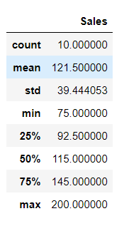
Use info() to get a concise summary of the DataFrame, including data types and non-null values. describe() provides statistical information such as mean, standard deviation, and quartiles for numeric columns.

# Display basic information about the DataFrame
df.info()

# Summary statistics for numeric columns
df.describe()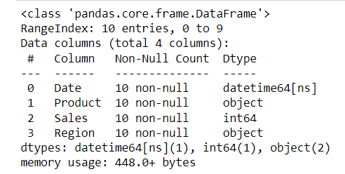

3. Handling Missing Data

These functions address missing data. dropna() removes rows with any missing values, while fillna() fills missing values with a specified value.

# Drop rows with missing values
df.dropna()

#Fill missing values with a specified value
df.fillna('NA')

4. Selecting Columns

Demonstrates selecting columns from the DataFrame. Use single brackets for a single column and double brackets for multiple columns.

# Select a single column
df['Product']

# Select multiple columns
df[['Product', 'Sales']]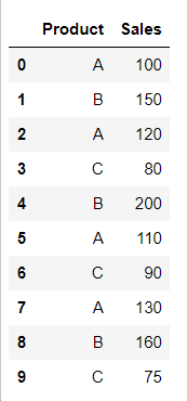

5. Filtering Data

Filtering allows you to extract rows based on conditions. The first example filters rows where sales are greater than 100. The second example introduces multiple conditions.

# Filter rows based on a condition
df[df['Sales'] > 100]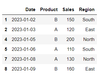

# Multiple conditions
df[(df['Region'] == 'North') & (df['Sales'] > 100)]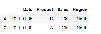

6. Sorting Data

Sorting the DataFrame based on a specific column (Sales in this case) in descending order.

# Sort DataFrame by a column
df.sort_values(by='Sales', ascending=False)

7. Grouping and Aggregating Data

Grouping data by a categorical column (Region) and calculating the mean of the 'Sales' column for each group.

# Group data by a column and calculate mean
df.groupby('Region')['Sales'].mean()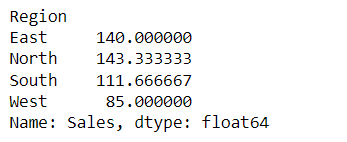

8. Applying Functions to Data

Using apply() to apply a custom function (doubling in this case) to each element in the 'Sales' column.

# Apply a function to each element in a column
df['Sales'].apply(lambda x: x * 2)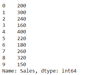

9. Concatenate DataFrames

Concatenating two DataFrames vertically (stacking them on top of each other).

# Concatenate DataFrames vertically
df2 = pd.concat([df, df])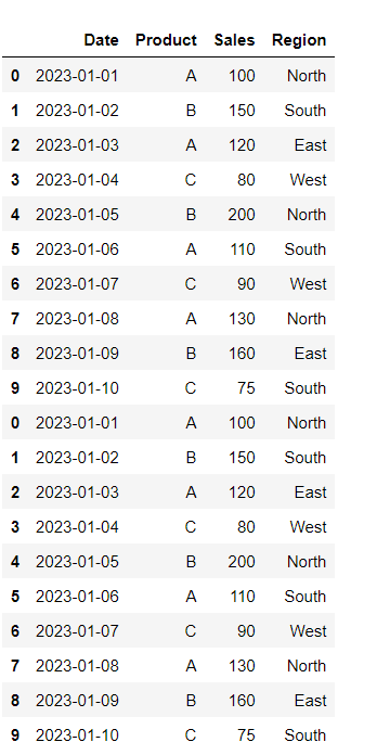

10. Handling Time Series Data

Converting a column containing date information to the datetime format and setting it as the DataFrame index, is crucial for time series analysis.

# Convert a column to datetime format
df['Date'] = pd.to_datetime(df['Date'])

# Set the datetime column as the index
df.set_index('Date', inplace=True)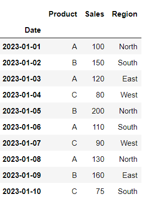

11. Resampling Time Series Data

Resampling time series data by month ('M') and calculating the mean. This is useful for changing the frequency of the data.

# Resample time series data by day
df.resample('M').mean()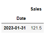

12. Creating New Columns

Creating a new column (‘Revenue’) by performing a calculation based on existing columns (here, multiplying ‘Sales’ by 1.2).

# Create a new column based on existing columns
df['Revenue'] = df['Sales'] * 1.2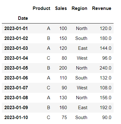

13. Removing Duplicates

Eliminating duplicate rows based on all columns. This is useful to ensure unique records in the DataFrame.

# Remove duplicate rows based on all columns
df.drop_duplicates()

14. Handling Text Data

Performing text operations. The first example converts text in the ‘Product’ column to lowercase. The second checks if each element contains the substring ‘A’.

# Convert text to lowercase
df['Product'].str.lower()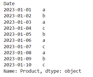

# Check for a substring in text
df['Product'].str.contains('A')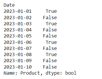

15. Handling Categorical Data

Converting a column to a categorical data type. This is beneficial for saving memory and improving performance when dealing with limited unique values.

# Convert a column to categorical
df['Region'] = pd.Categorical(df['Region'])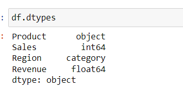

16. Pivot Tables

Creating a pivot table to summarize and analyze data. This example calculates the sum of sales for each combination of ‘Region’ and ‘Product’.

# Create a pivot table
pivot_table = pd.pivot_table(df, values='Sales', index='Region', columns='Product', aggfunc=np.sum)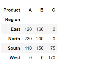

17. Merging DataFrames

Merging two DataFrames based on a common column (‘Region’ in this case) to combine information from both datasets.

# Merge two DataFrames
df2 = pd.DataFrame({'Region': ['North', 'South'], 'Manager': ['John', 'Jane']})
merged_df = pd.merge(df, df2, on='Region')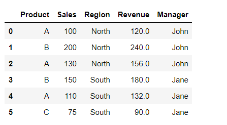

18. Calculating Cumulative Sum

Creating a new column (‘Cumulative_Sales’) to calculate the cumulative sum of the ‘Sales’ column over time.

# Calculate cumulative sum of a column
df['Cumulative_Sales'] = df['Sales'].cumsum()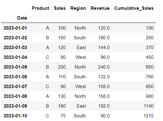

19. Rolling Statistics

Computing rolling statistics, such as the mean, over a specified window size (2 in this case). Useful for smoothing out fluctuations in time series data.

# Calculate rolling mean of a column
df['Rolling_Mean'] = df['Sales'].rolling(window=2).mean()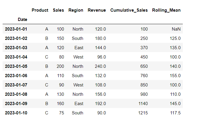

20. Handling Outliers

Identifying and replacing outliers in the ‘Sales’ column. Outliers beyond a certain threshold are replaced with the median value.

# Identify and replace outliers
upper_bound = df['Sales'].mean() + 2 * df['Sales'].std()
df['Sales'] = np.where(df['Sales'] > upper_bound, df['Sales'].median(), df['Sales'])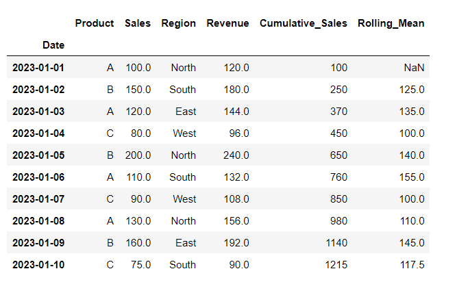

21. Shifting Data

Shifting values in the ‘Sales’ column by one period. Useful for comparing current and previous values.

# Shift values in a column
df['Shifted_Sales'] = df['Sales'].shift(periods=1)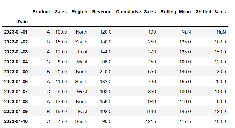

22. Calculating Percentage Changes

Computing the percentage change in the ‘Sales’ column. Useful for analyzing the rate of change between consecutive values.

# Calculate percentage change in a column
df['Percentage_Change'] = df['Sales'].pct_change() * 100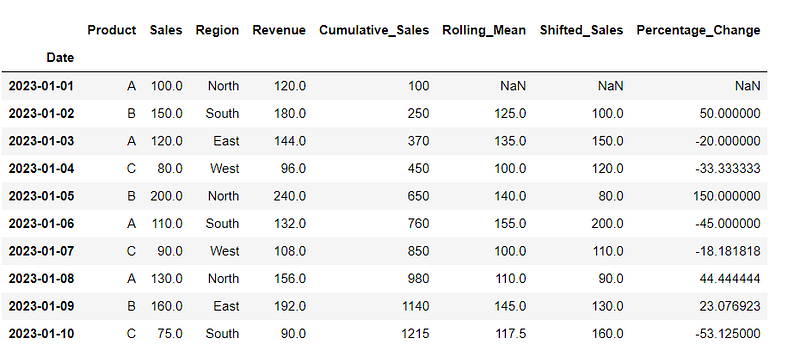

23. Correlation Matrix

Generating a correlation matrix to quantify the relationship between numeric variables in the DataFrame.

# Calculate correlation matrix
correlation_matrix = df.corr()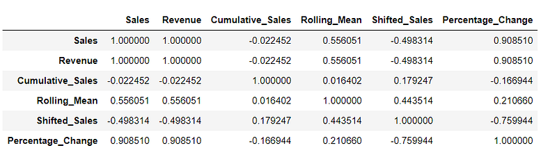

24. Plotting Data

Visualizing data by plotting the ‘Sales’ column as a line plot using Pandas and Matplotlib.

import matplotlib.pyplot as plt

# Plot data using Pandas
df['Sales'].plot(kind='line')
plt.show()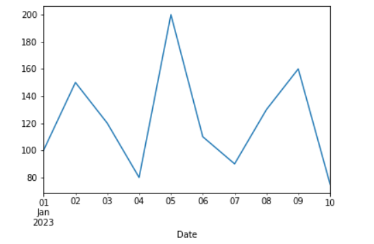

25. Saving Data

Saving the DataFrame to a CSV file for future use or sharing. The file will be stored in the same location as that of the python code.

# Save DataFrame to CSV file
df.to_csv('output_file.csv', index=False)

26. Memory Usage Optimization

Checking and optimizing the memory usage of the DataFrame to ensure efficient storage.

# Optimize memory usage
df.info(memory_usage='deep')

27. Custom Aggregation with agg

Using the agg function to apply custom aggregations to specific columns. In this example, we are calculating the sum of 'Sales' and the mean of 'Revenue'.

# Apply custom aggregation to columns
df.agg({'Sales': 'sum', 'Revenue': 'mean'})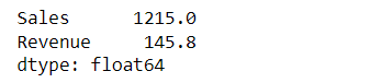

28. Binning Numeric Data

Binning numeric data (‘Sales’ column) into discrete intervals (bins) and labeling each interval accordingly.

# Create bins for numeric data
df['Sales_Bin'] = pd.cut(df['Sales'], bins=[0, 100, 150, 200], labels=['Low', 'Medium', 'High'])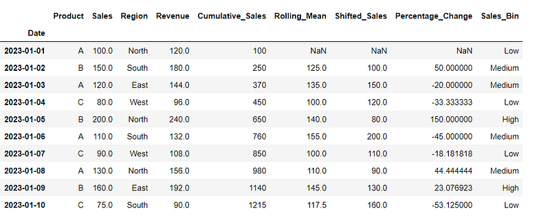

29. Finding Unique Values

Identifying unique values in the ‘Region’ column. Useful for understanding the distinct categories present in a categorical column.

# Find unique values in a column
unique_values = df['Region'].unique()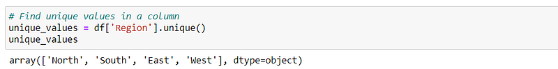

30. Value Counts

Counting the occurrences of each unique value in the ‘Region’ column. Useful for understanding the distribution of categorical data.

# Count occurrences of each value in a column
value_counts = df['Region'].value_counts()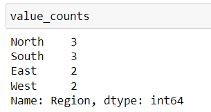

These examples showcase the application of various Pandas functions using a hypothetical sales dataset. Adapt and modify these code snippets based on your specific use case and dataset. Happy coding! 🐼🚀