Pairs trading with Ornstein-Uhlenbeck process (Part 2)

In this post I continue to implement and test strategies based on the the paper ‘Statistical Arbitrage in the U.S. Equities Market’ (Avellaneda and Lee, 2008). In the previous part I used just one industry ETF as a factor for decomposing stocks’ returns. Here I will try to use several ETFs as well as eigenportfolios calculated using Principal Component Analysis (PCA). I will also implement a modified version of the strategy that takes trading volume into account when calculating trading signals.

I will start with using more ETFs as factors in stock returns. As in the previous part I will trade the constituents of BBH ETF, but now I will also use another biotech ETF (IDNA) as well as SPY ETF as systematic risk factors. So each stock’s returns will be decomposed as:

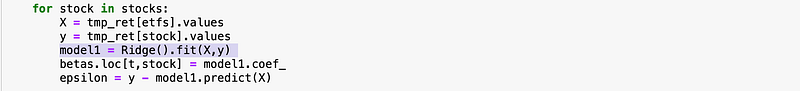
Since returns of ETFs can be strongly correlated, the usual linear regression might not always give stable results. To resolve this issue I’m going to use ridge regression, which is designed for datasets with highly correlated independent variables. It introduces additional regularization term which penalizes models with large coefficients.

The code is exactly the same as in the first part, just one line changes:

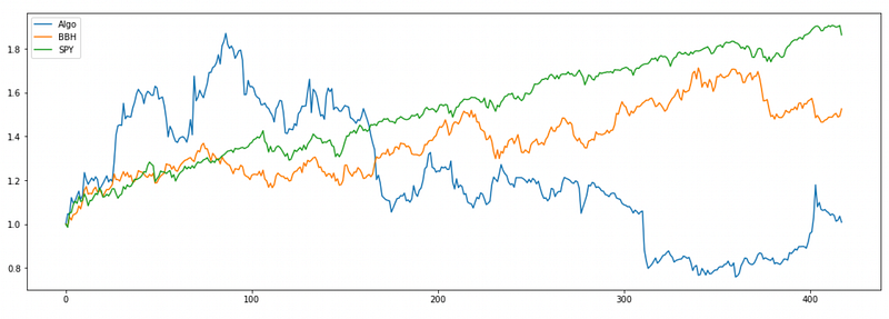
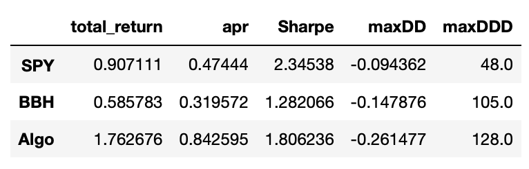
The results are provided below.

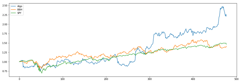
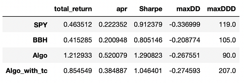
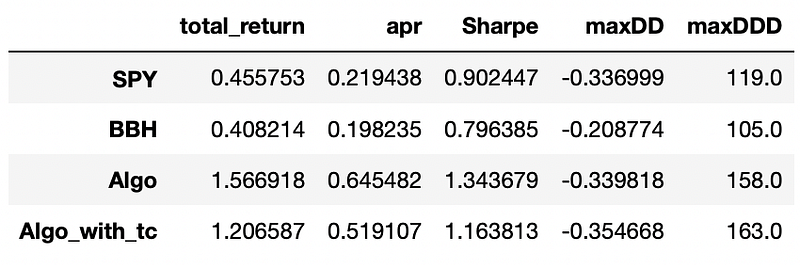
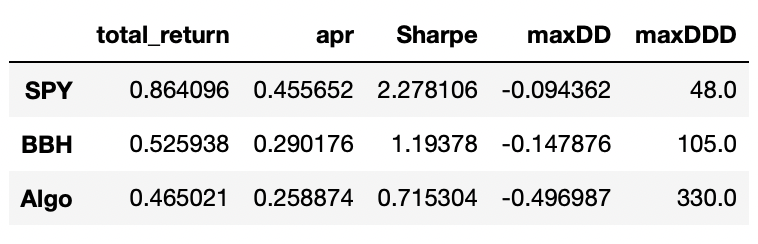
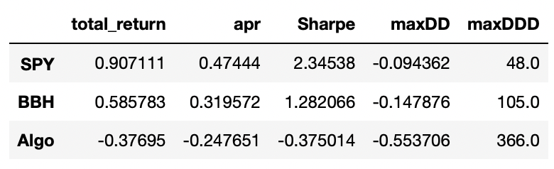
As a reminder here is the performance metrics we achieved in the previous part:

We can see that the only metric that is improved in the multiple ETF approach is maximum drawdown. Everything else was better before, when we used just one industry ETF as a risk factor. I think that this approach might be more suited for the situations when we want to trade stocks from a bigger universe covering multiple sectors and industries.

Now let’s look at the PCA approach. PCA is the method for finding the directions (principal components) of maximum variance in a given matrix, so that each component is orthogonal (perpendicular) to other components and components are not linearly correlated to each other. You can find many articles explaining in detail how PCA works (for example on wikipedia), but it is not really necessary to understand it. It can be done with one line of code in python.

What we need to do is to compute empirical correlation matrix of the given dataset and find its eigenvalues and eigenvector. Eigenvalues tell us how much variance is explained by a given component and the corresponding eigenvectors show us the direction of those components. Let me show you how this works in practice.

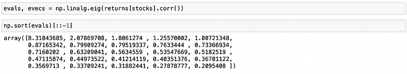
Above I calculate eigenvalues and eigenvectors of empirical correlation matrix of stocks’ returns. Then I print the eigenvalues in decreasing order. Each value tells us how much variance is explained by its corresponding component. If we divide it by the sum of all eigenvalues, we will get the fraction of variance explained.

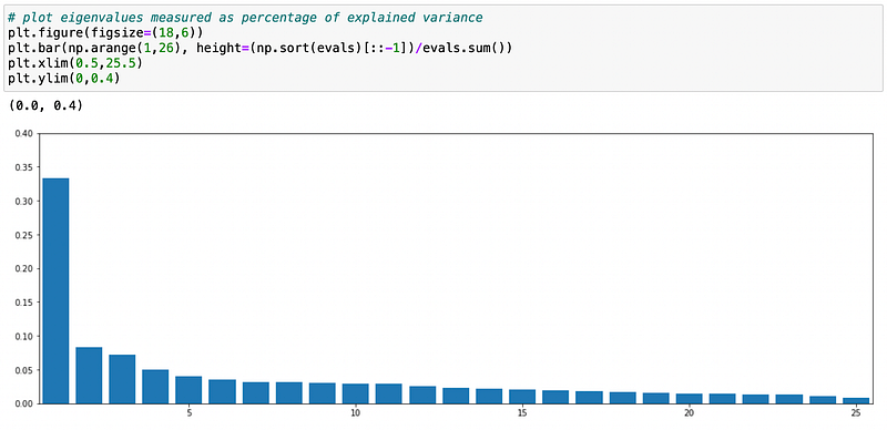
As you can see on the plot above, the first principal component (PC) explains a little less than 35% of total variance. Fraction of variance explained by the next components drops significantly.

What does that mean in application to stocks’ returns? It is said in the paper that the dominant eigenvector should be associated to the ‘market portfolio’. If we form a portfolio assigning weights proportional to the components of the dominant eigenvector and inversely proportional to corresponding stock volatility, it should have returns ‘similar’ to market returns. Let’s try to do it.

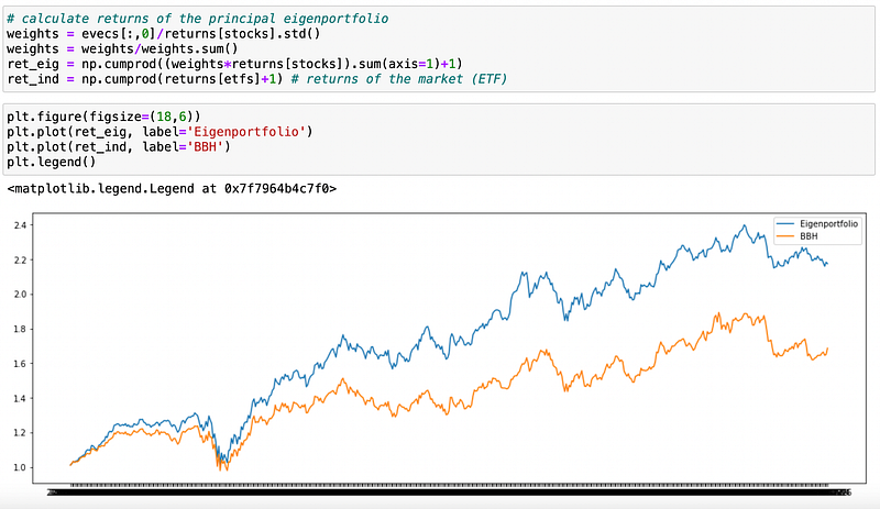
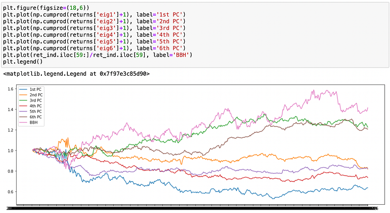
As we can see above, the two plots indeed look similar. Note that for the plot above I used the whole dataset to calculate eigenvalues and eigenvectors.

Next, authors claim that other eigenportfolios (corresponding to other eigenvectors) can be used as risk factors in decomposing returns. Basically everything is similar to the ETF approach, but now we are using eigenportfolios returns instead of ETFs returns.

Now we need to determine how many eigenportfolios should we use as risk factors. Below I will use 60 days rolling window to calculate the fraction of variance explained by the first component and by top5 components.

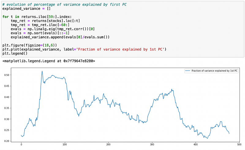
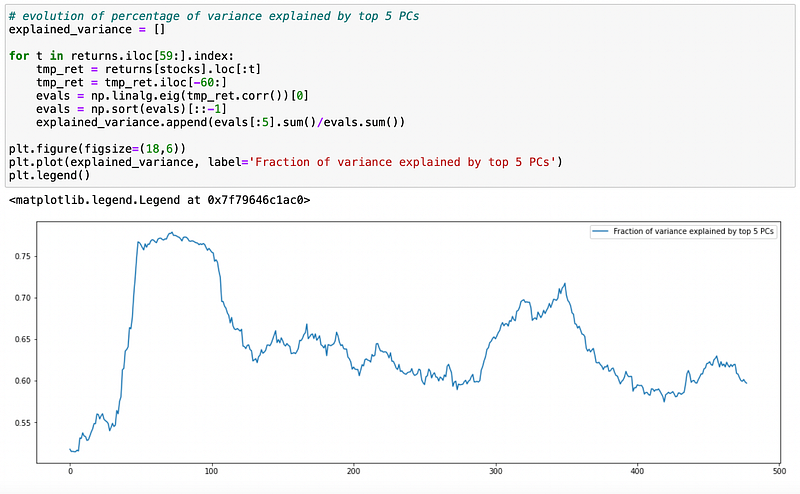
We can see that fraction of variance explained varies significantly. Let’s see how many components are required to explain at least 55% of total variance.

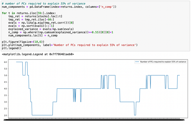
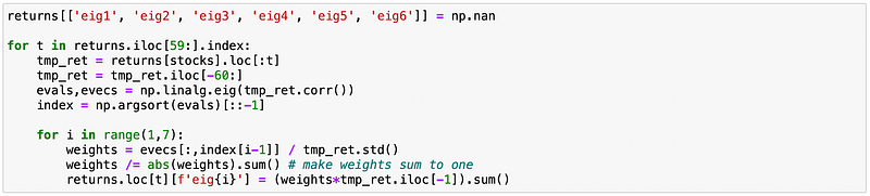
Number of principal components varies from 2 to 6 with average value around 4. Now I will compute and plot the returns of top 6 eigenportfolios.

Let’s look at the correlation matrix of returns.

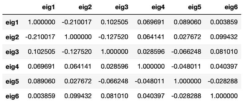
We can see that correlation coefficients between returns of different principal components are close to zero. This is exactly what we should expect after applying PCA.

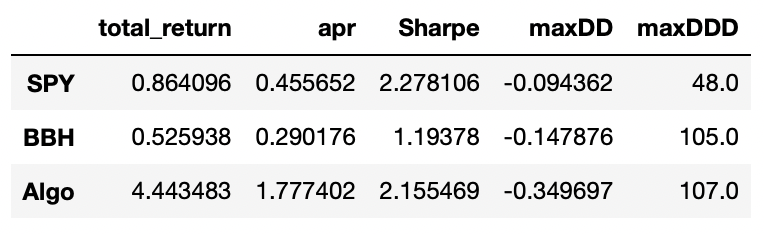
I backtested the strategy using one, four and six eigenportfolios as risk factors. Let’s look at the results.

One eigenportfolio:

Results look promising, but I didn’t account for any transaction costs here. Trading in eigenportfolios will have high transaction costs and it will probably consume a large fraction of the profits. But I think that the strategy might still be profitable. Now let’s see what happens when we increase the number of eigenportfolios.

Four eigenportfolios:

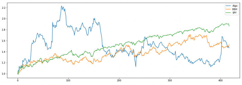
Very good start, but the end result is disappointing.

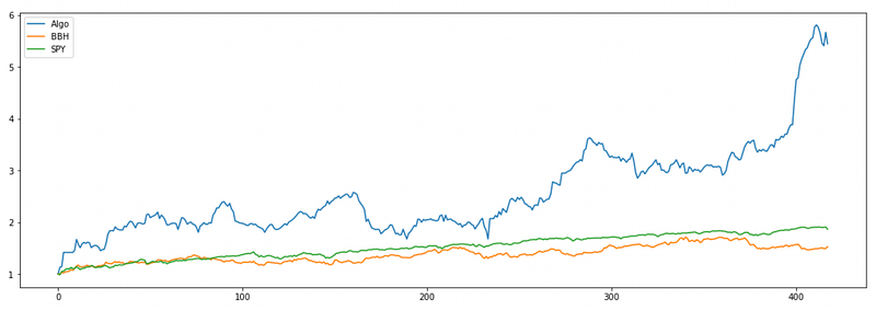
Six eigenportfolios:

This is even worse than before. Probably there is too much noise in those additional components.

Overall we see that only strategy with one eigenportfolio provides good results. Using larger number of eigenportfolios doesn’t provide any improvements and only decreases strategy performance. There are several possible reasons for it:

• Using more PCA components is more suitable when trading on a broader universe of stocks across multiple sectors\industries. Here we just have 25 stocks from one sector.
• The lookback window is too long (or too short). In the paper the strategy is tested on the data up to 2007 and they used 60 day lookback window. Maybe nowadays the markets are more dynamic and we should use shorter window.
• My implementation is wrong. Specifically I’m not sure that I correctly calculate the weights for eigenportfolios. When we have only long positions (when all the components of the eigenvector are nonnegative) everything is clear. But when we have both long and short positions I’m not sure how to calculate their weights. I assumed that the sum of absolute values of weights must be equal to one.

In part 6 of the paper authors explain how to take trading volume into account when making trading decisions. The idea is that the prices achieved on high volume are more trustworthy than the prices achieved on low volume. If the stock rises\falls on high volume, the chances are that it is due to the change in fundamentals and not due to market inefficiency, so entering short\long position is discouraged. On the other hand, if the volume is low, the chances of price discrepancy arising due to market inefficiency are higher. In that case we can be more certain that the price will revert back to its mean, so we enter a position.

Accounting for volume is really simple and done with one line of code:

We compute modified returns by multiplying the simple returns by the ratio of average volume over the last 60 days over the volume on a particular trading day. We then use modified returns in calculating s-scores.

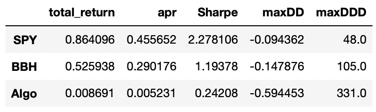
I tested this modification using 25 stocks and BBH ETF as a factor. The results are provided below:

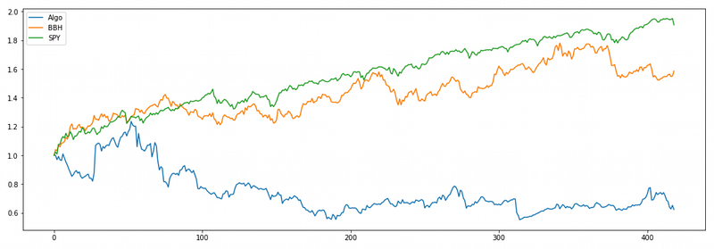
As you can see, the performance of such a strategy is really bad. So probably the assumption about prices achieved on high volume being more trustworthy is wrong.

When implementing this modification I accidentally tested a strategy with inverse modification: dividing the volume on a given day by the average volume. The strategy has very good performance:

Probably this performance is completely random, but I think that we can come up with a plausible explanation. Let’s assume that high trading volume indicates that investors are reacting to some new piece of information. It has been shown in some studies that investors tend to overreact to good or bad news. In that case, we should expect the stocks that move too much on high volume to revert back to their means. This is the opposite of what we assumed in the modification tested above. Of course this is explanation is just a speculation and needs to be properly tested.

The last tested strategy is the only one in this article that performs better than the baseline strategy implemented in the first part. But it was discovered by accident and needs to be further tested on different stocks and ETFs.

None of the other modifications tested here provide any improvement. I still think that these modifications might be useful if applied to different markets\assets, especially if we want to trade in a larger number of assets across different industries.

Jupyter notebook with source code is available here.

If you have any questions, suggestions or corrections please post them in the comments. Thanks for reading.

References

[1] Statistical Arbitrage in the U.S. Equities Market (Avellaneda and Lee, 2008)

Update 21.04.2022: There was a mistake in the PCA approach part of the article (thanks to hamasker for pointing it out). I fixed it now and updated the article and corresponding jupyter notebook.