Overview of Text Similarity Metrics in Python

Jaccard Index and Cosine Similarity — where you should use what, pros and cons of each.

While working on natural language models for search engines, I have frequently asked questions “How similar are these two words?”, “How similar are these two sentences?” , “How similar are these two documents?”. I have already talked about custom word embeddings in a previous post, where word meanings are taken into consideration for word similarity. In this blog post, we will look more into techniques for sentence or document similarity.

There are a few text similarity metrics but we will look at Jaccard Similarity and Cosine Similarity which are the most common ones.

Jaccard Similarity:

Jaccard similarity or intersection over union is defined as size of intersection divided by size of union of two sets. Let’s take example of two sentences:

Sentence 1: AI is our friend and it has been friendly Sentence 2: AI and humans have always been friendly

In order to calculate similarity using Jaccard similarity, we will first perform lemmatization to reduce words to the same root word. In our case, “friend” and “friendly” will both become “friend”, “has” and “have” will both become “has”. Drawing a Venn diagram of the two sentences we get:

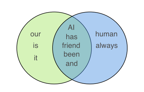
For the above two sentences, we get Jaccard similarity of 5/(5+3+2) = 0.5 which is size of intersection of the set divided by total size of set. The code for Jaccard similarity in Python is:

def get_jaccard_sim(str1, str2): 
    a = set(str1.split()) 
    b = set(str2.split())
    c = a.intersection(b)
    return float(len(c)) / (len(a) + len(b) - len(c))

One thing to note here is that since we use sets, “friend” appeared twice in Sentence 1 but it did not affect our calculations — this will change with Cosine Similarity.

Cosine Similarity:

Cosine similarity calculates similarity by measuring the cosine of angle between two vectors. This is calculated as:

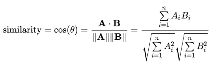
With cosine similarity, we need to convert sentences into vectors. One way to do that is to use bag of words with either TF (term frequency) or TF-IDF (term frequency- inverse document frequency). The choice of TF or TF-IDF depends on application and is immaterial to how cosine similarity is actually performed — which just needs vectors. TF is good for text similarity in general, but TF-IDF is good for search query relevance.

Another way is to use Word2Vec or our own custom word embeddings to convert words into vectors. I have talked about training our own custom word embeddings in a previous post.

There are two main difference between tf/ tf-idf with bag of words and word embeddings: 1. tf / tf-idf creates one number per word, word embeddings typically creates one vector per word. 2. tf / tf-idf is good for classification documents as a whole, but word embeddings is good for identifying contextual content.

Let’s calculate cosine similarity for these two sentences:

Sentence 1: AI is our friend and it has been friendly Sentence 2: AI and humans have always been friendly

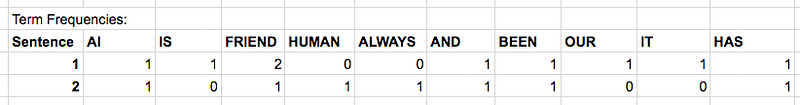
Step 1, we will calculate Term Frequency using Bag of Words:

Step 2, The main issue with term frequency counts shown above is that it favors the documents or sentences that are longer. One way to solve this issue is to normalize the term frequencies with the respective magnitudes or L2 norms. Summing up squares of each frequency and taking a square root, L2 norm of Sentence 1 is 3.3166 and Sentence 2 is 2.6458. Dividing above term frequencies with these norms, we get:

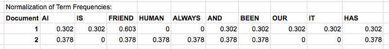
Step 3, as we have already normalized the two vectors to have a length of 1, we can calculate the cosine similarity with a dot product: Cosine Similarity = (0.302*0.378) + (0.603*0.378) + (0.302*0.378) + (0.302*0.378) + (0.302*0.378) = 0.684

Therefore, cosine similarity of the two sentences is 0.684 which is different from Jaccard Similarity of the exact same two sentences which was 0.5 (calculated above)

The code for pairwise Cosine Similarity of strings in Python is:

from collections import Counter
from sklearn.feature_extraction.text import CountVectorizer
from sklearn.metrics.pairwise import cosine_similarity
def get_cosine_sim(*strs): 
    vectors = [t for t in get_vectors(*strs)]
    return cosine_similarity(vectors)
    
def get_vectors(*strs):
    text = [t for t in strs]
    vectorizer = CountVectorizer(text)
    vectorizer.fit(text)
    return vectorizer.transform(text).toarray()

Differences between Jaccard Similarity and Cosine Similarity:

1. Jaccard similarity takes only unique set of words for each sentence / document while cosine similarity takes total length of the vectors. (these vectors could be made from bag of words term frequency or tf-idf)
2. This means that if you repeat the word “friend” in Sentence 1 several times, cosine similarity changes but Jaccard similarity does not. For ex, if the word “friend” is repeated in the first sentence 50 times, cosine similarity drops to 0.4 but Jaccard similarity remains at 0.5.
3. Jaccard similarity is good for cases where duplication does not matter, cosine similarity is good for cases where duplication matters while analyzing text similarity. For two product descriptions, it will be better to use Jaccard similarity as repetition of a word does not reduce their similarity.

If you know more applications for each, please mention in the comments below as it will help others. This concludes my blog on the overview of text similarity metrics. Good luck in your own explorations with text!

One of the best books I have found on the topic of information retrieval is Introduction to Information Retrieval, it is a fantastic book which covers lots of concepts on NLP, information retrieval and search.

I have started a new Substack where you can read more about my musings on ML, MLOps and LLMs. Follow me here to get articles right in your inbox.

If you have any questions, drop me a note at my LinkedIn profile. Thanks for reading!