Options trading data analysis — Part 1-An introduction

As an options trader, it is important to be able to monitor your performance and at the very least know whether or not your strategies are working and that you’re profitable. In the beginning, I tracked my trades using Excel, essentially keeping a record of each opening and closing trades. See figure 1. The numbers are obviously for example purposes only, but note the relationship between them.

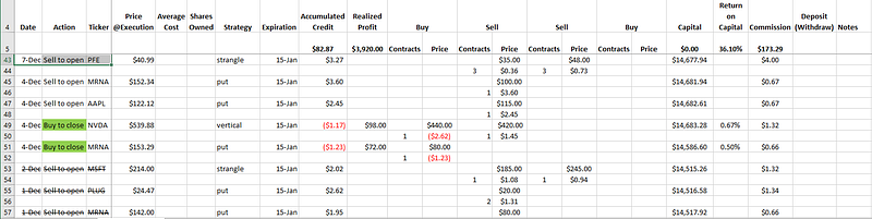
For opening trades, we record the price and number of contracts, where the price is recorded as a debit (negative) for buys and a credit (positive) for sells. Upon closing of the corresponding opening positions, we’ll once again sum the debits and credits and calculate the sum of the closing amount and the opening amount. This becomes our profit (where negative indicates a loss). The running capital is also tracked, as well as commission and fees for each trade. Return on capital is then calculated as the profit divided by the capital at closing (note that this is different from tracking buying power and calculating return based on buying power used). Coloring is used for closing transactions as a quick indicator of individual profit or loss. Opening transactions that had been closed will be shown with a strikethrough. Total profit and return on capital are also calculated as the sum of the corresponding columns and shown.

This certainly works for what it was, however, it is highly manual, hence time-consuming and tedious. Being a software developer, I have a propensity to seek better (lazier) ways.

The first thing I would want to do is to be able to get the transaction data directly from the broker, in order to avoid entering each manually. Most brokers allow users to download account transactions via CSV files. Even better if they provide API’s to obtain transactions in JSON format. At the time of writing, I know TD Ameritrade has a developer API to do just that: https://developer.tdameritrade.com/apis. I won’t go through the process of using any individual broker toolset to obtain transaction data here, but I will be working with the JSON provided by TD Ameritrade.

Once we are able to obtain transaction data, the next step is to set up our development environment. This is only done once. We will be using the Pandas library for Python, which is quite popular for data analysis. You can set up your own Python environment and install Pandas using pip. Jupyter Notebook is also convenient so install that as well (which can also be done using pip). Better yet though, if you’re up to it, head over to Colaboratory and everything is already ready to go. Convenient.

Now that our notebook is fired up, let’s get writing. The first thing we’d want to do is obviously include the necessary libraries and then load the transaction data file.

import json
import pandas as pd
from pandas.io.json import json_normalize

with open('transactions.json') as f:
    jsonData = json.load(f)

#by default normalization uses the '.' as the seperator 
# we're going to use the '_' instead
transactionsDf = pd.json_normalize(jsonData, sep='_')
transactionsDf = transactionsDf.iloc[::-1]

We’ll import json to deserialize to jsonData and then convert to a Pandas DataFrame. If we simply use transactionsDf = pd.DataFrame(jsonData), we’ll get a DataFrame that looks something like this:

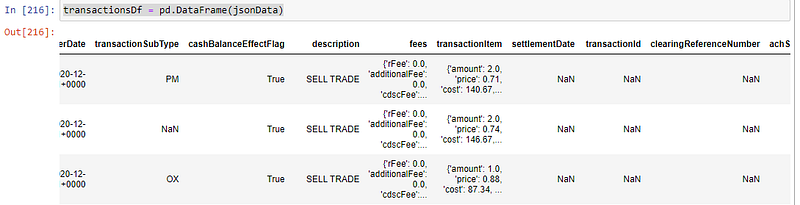
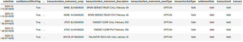
Note the nested objects for some column series. This isn’t very convenient when we want to utilize Pandas to perform data operations. Hence we import the json_normalize to “flatten” the data. TD Ameritrade also provides data that is sorted by date-time in descending order (going towards the past), we’ll also reverse the order for our DataFrame. Now we have something like this:

Running Capital and Principal

Now that the DataFrame is ready, the basic information of interest we’d want to calculate first is the running capital and principal, which will be the cumulative sum up to any given point. The way we define capital and principal will be:

• capital — the total cash equivalent amount at a given moment
• principal — the total contributed cash equivalent amount at a given moment

Capital will essentially be principal + gains. For TD Ameritrade, the change in capital is recorded in the netAmount field for each transaction. We do, however, want to exclude transactions that are related to their cash sweep program. Pandas has a built-in function to calculate the cumulative sum that we can utilize.

transactionsDf= transactionsDf.assign(capital = transactionsDf.apply(
    lambda row : row['netAmount'] 
    if (str.upper(row['type']) != 'JOURNAL' and str.upper(row['description']) != 'CASH ALTERNATIVES PURCHASE') else 0, axis=1).cumsum())

First, we use the apply function on the DataFrame, iterating through each row (axis=1)to filter out the mentioned transactions we wanted to exclude, returning 0 for those and netAmount otherwise. This results in a dataframe with a single column with the netAmount. We then run this through the cumsum function and append it to the transactionDf dataframe as thecapital column using the assign function.

As for the principal, we’re interested in deposit and withdrawal transactions. These can be identified with the ELECTRONIC_FUND as the type and transactionSubType of FI and FO. Deposits are straightforward as they add directly to the current principal. However, we need to be a bit careful with withdrawals. If there are gains, the withdrawal will need to be applied to the gain before it is applied to the principal, if at all. Because of this, the calculation of the principal has a dependency on the capital. If we simply just add everything, we can get undesirable results, as demonstrated by this simplified example:

    Type    Amount  Capital Principal
0   D       10      10      10
1   D       10      20      20
2   W       -5      15      15
3   D       10      25      25
4   G       5       30      25
5   G       5       35      25
6   G       5       40      25
7   L       -5      35      25
8   W       -10     25      15   <- should stays at 25
9   G       10      35      15   <- now wrong because of above
10  W       -25     10      -10  <- error escalades
11  G       25      35      -10
12  L       -30     5       -10

We must mind the caveat and calculate the principal by iterating through each row.

#calculate the running principal
# for withdrawals, we only subtract from the principal only when capital will fall below principal
# this is because if capital is above principal, then the withdrawals would be taking out of the "gains"

transactionsDf['principal'] = np.nan
currentPrincipal = 0

for index, row in transactionsDf.iterrows():
    if (row['type'] == 'ELECTRONIC_FUND'):
        if (row['capital'] <= currentPrincipal):
            transactionsDf.loc[index, 'principal'] = row['capital']
        else:
            transactionsDf.loc[index, 'principal'] = currentPrincipal + row['netAmount']
    else:
        transactionsDf.loc[index, 'principal'] = currentPrincipal

    currentPrincipal = transactionsDf.loc[index, 'principal']

Note, for this we use loc to “assign” the principal one row at a time. And finally, in a notebook, we can select to view the principal and capital using the loc once again: transsactionDf.loc[:0,[‘capital’, ‘principal’]].

By this point, we are able to get the first glimpse of our performance over time, by comparing principal and capital. Essentially, the delta between capital and principal would be our realized profit. In a later part of this series, we will expand what we have to calculate profit and loss for each closing trade and explore techniques to group such data to provide relevant views for analysis.

Part 2 — Visuals