Option Valuation: A Comparison of The Merton Jump Diffusion Model And Bjerksund Stensland

Option valuation models play a crucial role in financial markets, enabling investors and traders to determine the fair value of options. These models provide insights into the pricing of financial derivatives, specifically options, which are contracts that grant the holder the right, but not the obligation, to buy or sell an underlying asset at a predetermined price (the strike price) within a specific time frame. In this article, we will delve into two prominent option valuation models: the Merton Jump Diffusion Model and the Bjerksund Stensland Model. By understanding their differences and applications, traders can make more informed investment decisions.

Option Valuation and Its Importance

Option valuation refers to the process of determining the fair value of an option contract. It involves assessing various factors, such as the underlying asset’s price, time to expiration, volatility, risk-free interest rate, and dividend yield (if applicable). By valuing options, traders can assess whether they are overpriced, underpriced, or fairly priced in the market. This information is invaluable for constructing trading strategies, risk management, and identifying arbitrage opportunities.

The Role of Option Valuation for Traders

Option valuation models provide traders with valuable insights and tools for decision-making. By accurately pricing options, traders can identify mispriced options and potentially exploit arbitrage opportunities. Additionally, option valuation models help traders assess the potential risk and reward associated with different options strategies. These models enable traders to hedge their positions effectively, manage risk exposure, and optimize their portfolio allocation.

Historical, Implied, and Future Volatility

Volatility is a critical factor in option valuation, representing the measure of price fluctuation for the underlying asset. Traders consider different types of volatility when valuing options.

1. Historical Volatility: Historical volatility measures the standard deviation of the underlying asset’s price returns over a specific period. It provides insights into past price movements and is calculated using historical data. This information helps traders assess the asset’s past volatility patterns.
2. Implied Volatility: Implied volatility reflects the market’s expectation of future price volatility. It is derived from the options’ market prices and reflects the market participants’ sentiment regarding potential future price swings. Implied volatility is an essential input in option valuation models, allowing traders to estimate the options’ fair value.
3. Future Volatility: Future volatility represents the unknown volatility of the underlying asset during the option’s lifespan. It plays a crucial role in determining the option’s value and is typically estimated using option pricing models.

Black & Scholes Model and Alternative Models

The Black & Scholes Model is one of the most widely recognized option valuation models. It assumes that the underlying asset follows geometric Brownian motion, with constant volatility and no jumps in prices. While this model provides a solid foundation for option valuation, it may not capture certain market dynamics accurately.

To address the limitations of the Black & Scholes Model, alternative models, such as the Merton Jump Diffusion Model and the Bjerksund Stensland Model, have been developed. These models introduce additional parameters and assumptions to incorporate more realistic market behavior.

Merton Jump Diffusion Model

The Merton Jump Diffusion Model is an extension of the Black & Scholes Model that accounts for sudden jumps in asset prices. It incorporates a Poisson process to model these discontinuous price movements. This model assumes that the underlying asset’s returns consist of both a continuous diffusion component and a jump component. The jumps follow a log-normal distribution and occur randomly with a known average frequency.

The Merton Jump Diffusion Model provides a more accurate representation of market behavior by considering the occurrence of large price jumps. It captures extreme events that the Black & Scholes Model cannot account for, making it suitable for valuing options on assets with significant price jump risk.

Here is the Python code with the Merton Jump Diffusion Model implementation.

# Converted and tested from https://github.com/AnthonyBradford/optionmatrix/blob/master/src/models/metaoptions/src/JumpDiffusion.c
import math
import numpy as npdef cnd(x):
    a1 = 0.31938153
    a2 = -0.356563782
    a3 = 1.781477937
    a4 = -1.821255978
    a5 = 1.330274429

L = abs(x)
    K = 1.0 / (1.0 + (0.2316419 * L))
    a12345k = (a1 * K) + (a2 * K * K) + (a3 * K * K * K) + (a4 * K * K * K * K) + (a5 * K * K * K * K * K)
    result = 1.0 - (1.0 / math.sqrt(2 * math.pi)) * math.exp(-L**2 / 2.0) * a12345k
    if x < 0.0:
        result = 1.0 - result
    return result
def gbs_call(S, X, T, r, b, v):
    vst = v * math.sqrt(T)
    d1 = (math.log(S / X) + (b + v**2 / 2) * T) / vst
    return S * math.exp((b - r) * T) * cnd(d1) - X * math.exp(-r * T) * cnd(d1 - vst)
def gbs_put(S, X, T, r, b, v):
    vst = v * math.sqrt(T)
    d1 = (math.log(S / X) + (b + v**2 / 2) * T) / vst
    return X * math.exp(-r * T) * cnd(-(d1 - vst)) - S * math.exp((b - r) * T) * cnd(-d1)
# Parameters
#   S: Price of underlying asset
#   X: Exercise price of the option
#   T: Time to expiration in years (ie. 33 days to expiration is 33/365)
#   r: Risk free rate (ie. 2% is 0.02)
#   v: Volatility percentage (ie. 30% volatility is 0.30)
#   lambda_val: The jump rate
#   gamma_val: The jump size
def jump_diffusion(isCall, S, X, T, r, v, lambda_val, gamma_val):
    fact_lookup = [
        1,
        1,
        2,
        6,
        24,
        120,
        720,
        5040,
        40320,
        362880,
        3628800
    ]
    try:
        elT = math.exp(-lambda_val * T)
        p2v = v**2
        p2delta = (math.sqrt(gamma_val * p2v / lambda_val))**2
        p2Z = (math.sqrt(p2v - lambda_val * p2delta))**2
        result = 0.0
        for i in range(11):
            vi = math.sqrt(p2Z + p2delta * (i / T))
            if isCall:
                bs = gbs_call(S, X, T, r, r, vi)
            else:
                bs = gbs_put(S, X, T, r, r, vi)
            result += elT * (lambda_val * T)**i / fact_lookup[i] * bs
    except:
        result = np.NaN
    return result

Bjerksund Stensland Model

The Bjerksund Stensland Model is another option valuation model that improves upon the Black & Scholes Model. This model allows the early exercise of American options, which can be exercised before their expiration date. The Bjerksund Stensland Model incorporates a closed-form solution for pricing American options on assets that pay dividends and can handle stochastic interest rates.

This model is particularly useful when valuing options that can be exercised early, providing flexibility to traders. It accounts for various factors, such as dividend payments, which are prevalent in real-world scenarios, making it a valuable tool for option valuation.

Here is the Python code implementing the Bjerksund Stensland model.

from math import * 

def cdf(x):
    return (1.0 + erf(x / sqrt(2.0))) / 2.0

def phi(s, t, gamma, h, i, r, a, v):
    lambda1 = (-r + gamma * a + 0.5 * gamma * (gamma - 1) * v**2) * t
    dd = -(log(s / h) + (a + (gamma - 0.5) * v**2) * t) / (v * sqrt(t))
    k = 2 * a / (v**2) + (2 * gamma - 1)

    try:
        return exp(lambda1) * s**gamma * (cdf(dd) - (i / s)**k * cdf(dd - 2 * log(i / s) / (v * sqrt(t))))
    except OverflowError as err:
        return exp(lambda1) * s**gamma * cdf(dd)

# Call Price based on Bjerksund/Stensland Model
# Parameters
#   underlying_price: Price of underlying asset
#   exercise_price: Exercise price of the option
#   time_in_years: Time to expiration in years (ie. 33 days to expiration is 33/365)
#   risk_free_rate: Risk free rate (ie. 2% is 0.02)
#   volatility: Volatility percentage (ie. 30% volatility is 0.30)
def bjerksund_stensland_call(underlying_price, exercise_price, time_in_years, risk_free_rate, volatility):
    div = 1e-08
    z = 1
    rr = risk_free_rate
    dd2 = div
    
    dt = volatility * sqrt(time_in_years)
    drift = risk_free_rate - div
    v2 = volatility**2
    
    b1 = sqrt((z * drift / v2 - 0.5)**2 + 2 * rr / v2)
    beta = (1 / 2 - z * drift / v2) + b1
    binfinity = beta / (beta - 1) * exercise_price
    bb = max(exercise_price, rr / dd2 * exercise_price)
    ht = -(z * drift * time_in_years + 2 * dt) * bb / (binfinity - bb)
    i = bb + (binfinity - bb) * (1 - exp(ht))

    if underlying_price < i and beta < 100:
        alpha = (i - exercise_price) * i**(-beta)
        return alpha * underlying_price**beta - alpha * phi(underlying_price, time_in_years, beta, i, i, rr, z * drift, volatility) + phi(underlying_price, time_in_years, 1, i, i, rr, z * drift, volatility) - phi(underlying_price, time_in_years, 1, exercise_price, i, rr, z * drift, volatility) - exercise_price * phi(underlying_price, time_in_years, 0, i, i, rr, z * drift, volatility) + exercise_price * phi(underlying_price, time_in_years, 0, exercise_price, i, rr, z * drift, volatility)
    
    return underlying_price - exercise_price

# Put Price based on Bjerksund/Stensland Model
# Parameters
#   underlying_price: Price of underlying asset
#   exercise_price: Exercise price of the option
#   time_in_years: Time to expiration in years (ie. 33 days to expiration is 33/365)
#   risk_free_rate: Risk free rate (ie. 2% is 0.02)
#   volatility: Volatility percentage (ie. 30% volatility is 0.30)
def bjerksund_stensland_put(underlying_price, exercise_price, time_in_years, risk_free_rate, volatility):
    div = 1E-08
    z = -1
    rr = div
    dd = rr
    dd2 = 2 * dd - rr
    asset_new = underlying_price
    underlying_price = exercise_price
    exercise_price = asset_new

    dt = volatility * sqrt(time_in_years)
    drift = risk_free_rate - div
    v2 = volatility**2

    b1 = sqrt((z * drift / v2 - 0.5)**2 + 2 * rr / v2)
    beta = (1 / 2 - z * drift / v2) + b1
    binfinity = beta / (beta - 1) * exercise_price
    bb = max(exercise_price, rr / dd2 * exercise_price)
    ht = -(z * drift * time_in_years + 2 * dt) * bb / (binfinity - bb)
    i = bb + (binfinity - bb) * (1 - exp(ht))
        
    if underlying_price < i and beta < 100:
        alpha = (i - exercise_price) * i**(-beta)
        return alpha * underlying_price**beta - alpha * phi(underlying_price, time_in_years, beta, i, i, rr, z * drift, volatility) + phi(underlying_price, time_in_years, 1, i, i, rr, z * drift, volatility) - phi(underlying_price, time_in_years, 1, exercise_price, i, rr, z * drift, volatility) - exercise_price * phi(underlying_price, time_in_years, 0, i, i, rr, z * drift, volatility) + exercise_price * phi(underlying_price, time_in_years, 0, exercise_price, i, rr, z * drift, volatility)
    
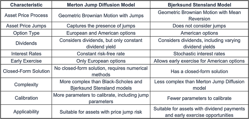
    return underlying_price - exercise_price

Merton Jump Diffusion Model vs. Bjerksund Stensland Model

Below is a comparison table highlighting the main characteristics of the Merton Jump Diffusion Model and the Bjerksund Stensland Model

Conclusion

In conclusion, both the Merton Jump Diffusion Model and the Bjerksund Stensland Model offer valuable enhancements to the traditional Black & Scholes Model for option valuation. The Merton Jump Diffusion Model incorporates jumps in asset prices, capturing extreme events and assets with price jump risk. On the other hand, the Bjerksund Stensland Model allows the early exercise of American options and handles dividends and stochastic interest rates.

The choice between the two models depends on the specific characteristics of the options being valued. Traders should consider factors such as the presence of price jumps, dividend payments, and the flexibility of early exercise. By carefully assessing these factors and understanding the nuances of each model, traders can make more informed decisions regarding option valuation and trading strategies.

If you enjoy my work, please support me on Medium by becoming a member through my referral link, and consider giving it a clap as a small gesture of motivation. Thank you!

Twitter / X: https://twitter.com/diegodegese LinkedIn: https://www.linkedin.com/in/ddegese Github: https://github.com/crapher

Disclaimer: Investing in the stock market involves risk and may not be suitable for all investors. The information provided in this article is for educational purposes only and should not be construed as investment advice or a recommendation to buy or sell any particular security. Always do your own research and consult with a licensed financial advisor before making any investment decisions. Past performance is not indicative of future results.